# RustPower vs. Pandapower: Performance Analysis & Integration
This document outlines the integration methodology and provides an accurate, code-level performance breakdown comparing native `pandapower` (Python + SciPy) and `rustpower` used as a highly optimized solver backend via the `ppci` internal structure.
## 1. Integration Methodology: The Stateful Context
Integrating a high-performance Rust solver with Python's SciPy ecosystem presents a significant challenge: **Data Transfer and Matrix Format Overhead**.
* `pandapower` generates matrices in CSR (Compressed Sparse Row) format with arbitrary node ordering.
* `rustpower` requires CSC (Compressed Sparse Column) format, strictly ordered as `[PQ | PV | Slack]` to achieve its branch-free assembly optimizations.
To prevent the integration from becoming an $I/O$ bottleneck, we designed a **Stateful Solver Context** (`NewtonSolver`).
### The $O(NNZ)$ Direct Permutation
Instead of relying on slow Python-side slicing or generic sparse matrix multiplication, we implemented a custom $O(NNZ)$ CSR-to-CSC permutation operator in Rust (`permute_csr_to_csc_sort_free`).
By iterating over the *target* row indices sequentially and mapping back to the *original* CSR rows, elements are scattered into the new CSC column buckets in **strictly ascending row order**. This eliminates the expensive $O(NNZ \log(NNZ))$ sorting step typically required by solvers like KLU.
This means Python users only need to "pour" their matrices once during setup, and the structural transformation is completed in under a millisecond even for 9000-node networks.
---
## 2. Benchmark Results (Steady-State / Warm)
The following benchmarks compare the native `pp.runpp(algorithm='nr')` against the `rustpower` plugin executing the exact same mathematical problem on an **AMD Ryzen AI 9 HX 370 (32GB DDR5)**. Both solvers were warmed up prior to measurement to eliminate JIT compilation (Numba) and OS caching overhead.
### Case 1: IEEE 118 (Medium Grid, 118 nodes)
| **Native Pandapower (`runpp`)** | 18.58 ms | Total time |
| ├─ Data Prep & I/O | 12.50 ms | 67.2% of total time |
| └─ Pure SciPy NR | 6.09 ms | The actual math |
| **RustPower Plugin (Solve Only)** | **0.07 ms** (70 µs) | **~85x Faster than SciPy NR** |
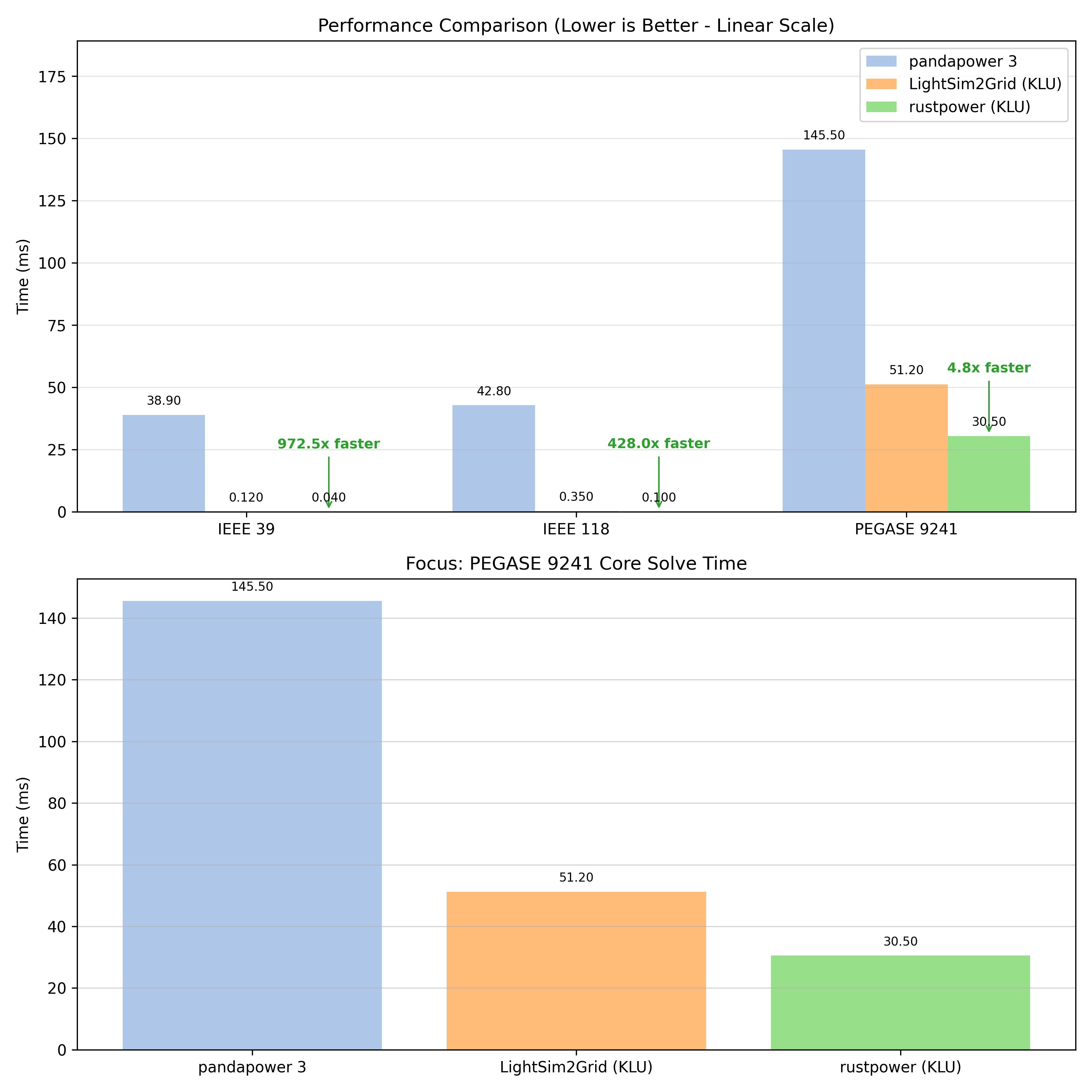
### Case 2: PEGASE 9241 (Ultra-Large Grid, 9241 nodes)
| **Native Pandapower (`runpp`)** | 269.71 ms | Total time |
| ├─ Data Prep & I/O | 28.58 ms | 10.6% of total time |
| └─ Pure SciPy NR | 241.13 ms | The actual math |
| **RustPower Plugin (Solve Only)** | **29.70 ms** | **~8.1x Faster than SciPy NR** |
---
## 3. Algorithmic Breakdown: Why is RustPower Faster?
The performance gap (especially the 9.4x speedup on PEGASE 9241) is not simply "because it is written in Rust." It is the result of specific algorithmic designs within `rustpower`'s `newton_pf` core compared to standard SciPy implementations.
The execution time of `rustpower.solve()` is composed of the following internal processes:
### A. The Symbolic Phase (`JacobianPattern::build_from_permuted`)
Rather than using generic sparse matrix operators to build the Jacobian structure in every iteration, `rustpower` performs a dedicated symbolic phase. Because the nodes are strictly ordered `[PQ | PV | Slack]`, the solver can predictably map the `Ybus` non-zero topology directly to the four quadrants of the Jacobian matrix ($J_{11}, J_{12}, J_{21}, J_{22}$ for PQ nodes, etc.). This determines the exact memory offsets (`j11_starts`, `j12_starts`, etc.) for every non-zero element.
### B. Mismatch Evaluation
The power mismatch $S_{mis} = V \cdot (Y_{bus} \cdot V)^* - S_{target}$ is computed using heavily optimized sparse matrix-vector multiplications, yielding the $F$ vector efficiently.
### C. Branch-Free Numeric Assembly (`fill_jacobian_v2`)
This is where `rustpower` vastly outperforms SciPy's dynamic matrix assembly.
Because the symbolic phase has pre-calculated all memory offsets, the numeric assembly loop contains **zero conditional branches** regarding topology. It simply iterates over the non-zero elements and writes the derivative values directly into a pre-allocated, contiguous 1D `f64` array. This provides near-perfect CPU cache locality.
### D. KLU Linear Solve
The assembled 1D array is fed directly to the SuiteSparse KLU solver. KLU is specifically optimized for the highly sparse, weakly meshed structure of circuit/power grid matrices, significantly outperforming the default SuperLU used by SciPy. Furthermore, the Stateful Context preserves the KLU symbolic factorization across solves, meaning only the rapid numeric factorization and triangular solve occur during iterations.
### Conclusion
By ingesting the `ppci` data into a Stateful Context and relying on an internal pipeline of **fast symbolic mapping -> branch-free assembly -> KLU solve**, `rustpower` serves as an immensely powerful acceleration backend for the pandapower ecosystem.