# Migrating from plotters
[plotters](https://crates.io/crates/plotters) gives you a drawing area and
primitives; rizzma gives you matplotlib's plotting vocabulary. Most plotters
code in scientific projects hand-rolls things rizzma already ships: images
drawn pixel by pixel, colormap tables copied between files, contours faked by
marking cells, histograms binned by hand. This guide maps plotters concepts to
rizzma, ports the ten idioms that come up most, and works through a real
program end to end.
Every rizzma snippet below is compiled and run as a doc test, and draws the
image shown beside it in the gallery. The plotters snippets are for reference
only.
## Concept map
| `BitMapBackend::new(path, (w, h)).into_drawing_area()` | `Figure::new(width_in, height_in)` (100 DPI by default; `with_dpi`) |
| `root.fill(&WHITE)` | nothing: figures start white (`RcParams` for themes) |
| `ChartBuilder::on(&root)…build_cartesian_2d(x0..x1, y0..y1)` | `fig.add_subplot(1, 1, 1)`; limits autoscale, or `set_xlim` / `set_ylim` |
| `.caption(text, font)` | `ax.set_title(text)`; `fig.suptitle(text)` above every panel |
| `.margin`, `.x_label_area_size`, `.y_label_area_size` | nothing: tight layout measures ticks and labels |
| `root.split_evenly((r, c))` | `fig.add_subplot(r, c, i)`, or a `GridSpec` for ratios and spans |
| `configure_mesh().x_desc(..).y_desc(..)` | `ax.set_xlabel(..)`, `ax.set_ylabel(..)` |
| `configure_mesh().x_labels(n)`, `.disable_mesh()` | `ax.set_xticks(&[..])`, `ax.grid(true)` (grids start off) |
| `draw_series(LineSeries::new(points, style))` | `ax.plot(&x, &y)` (returns the `Line2D` to restyle) |
| `draw_series(points.map(Circle::new(..)))` | `ax.scatter(&x, &y)` (returns the `Collection`) |
| `.label(..).legend(..)` + `configure_series_labels()` | `line.set_label(..)` + `ax.legend_auto()` |
| `root.present()` | `fig.save_png(path)`, `fig.save_svg(path)`, `fig.save_pdf(path)` |
| `BitMapBackend::with_buffer(&mut buf, (w, h))` | `fig.render_into(&mut buf, PixelFormat::Rgba8)`, `fig.encode_png()` |
Colors come from matplotlib's default cycle, so successive `plot` calls need
no color bookkeeping.
## Naming traps from matplotlib
- matplotlib's bare `ax.legend()` collects labelled artists; in rizzma that is
`ax.legend_auto()`. rizzma's `ax.legend(entries)` takes explicit
`(Rgba, String)` rows.
- Methods that add an artist return it: `ax.plot(..)` gives a `&mut Line2D`,
`ax.scatter(..)` a `&mut Collection`, `ax.imshow(..)` a `&mut AxesImage`, so
you style it in place: `ax.plot(&x, &y).set_label("fit").set_linewidth(2.0)`.
Builder methods named `with_*` consume a value you construct yourself;
`set_*` methods restyle in place.
- `set_aspect("equal")` is `set_aspect_equal()`, and scales are
`set_xscale_log(10.0)` and friends rather than strings.
- A colorbar names what it describes: `ax.colorbar(Mappable::Image(0))`, the
first image of that axes, instead of a returned handle.
- `twinx` is on the figure and returns the new axes' index:
`let right = fig.twinx(0); fig.axes_mut()[right].plot(..)`.
## Colormaps: the default, and what replaces jet
Two differences from matplotlib matter when you port colored plots:
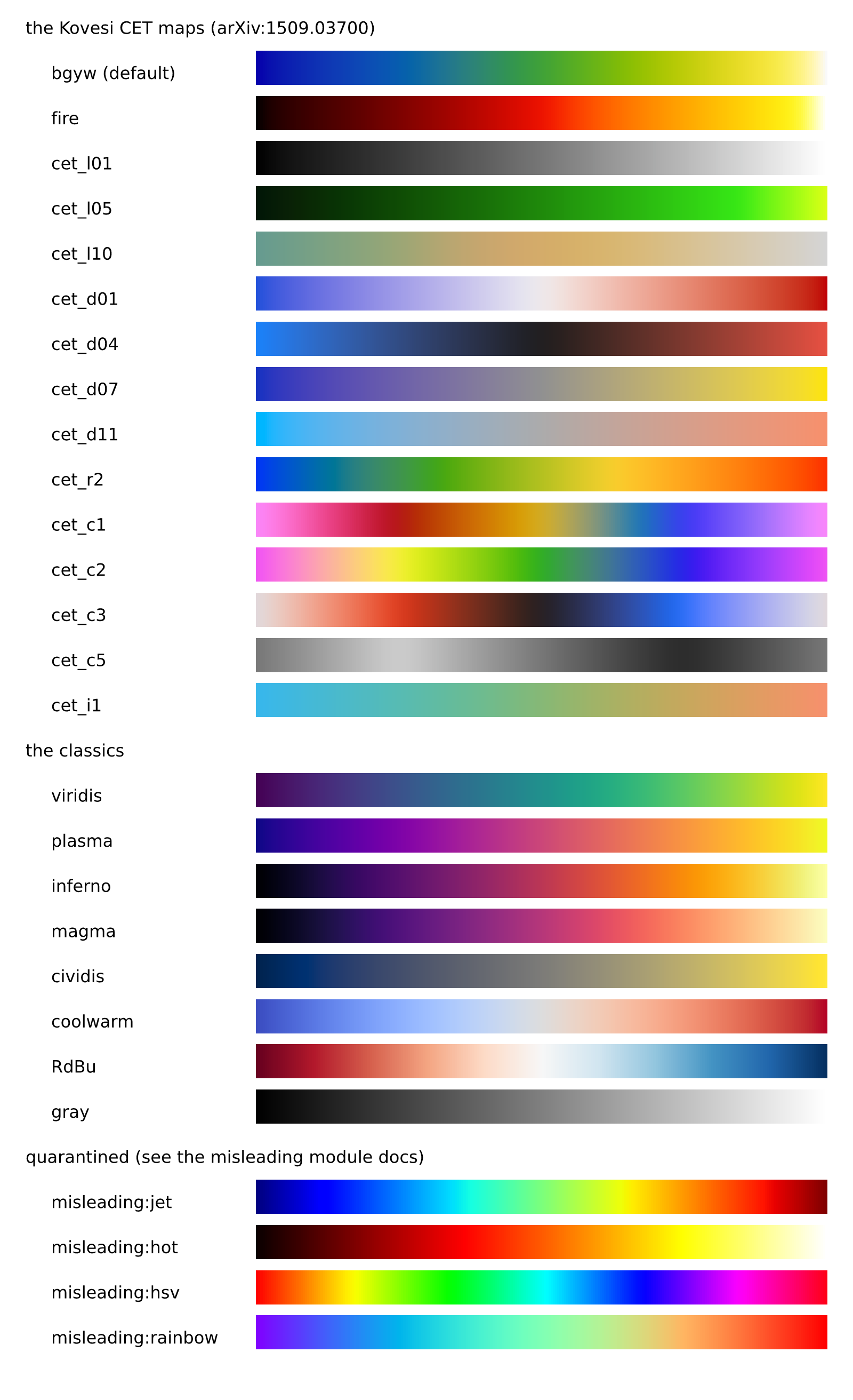
- **The default colormap is `bgyw`** (CET-L09, a perceptually uniform
blue-green-yellow-white), not matplotlib's viridis. Any call that takes no
colormap (`imshow`, `pcolormesh`, `contourf`, …) uses it. Name `"viridis"`
where you need matplotlib's look; viridis, magma, inferno, plasma,
cividis, gray, RdBu and coolwarm are all here, each with an `_r` reversed
variant.
- **jet, hot, hsv and rainbow are quarantined.** Their lightness profiles
invent edges and hide features (Kovesi, *Good Colour Maps*), so the bare
names don't resolve. Each has an honest replacement, and the original
stays reachable behind a `misleading:` prefix for exact reproduction.
| `jet`, `rainbow` | `"cet_r2"` | `"misleading:jet"`, `"misleading:rainbow"` |
| `hot` | `"cet_l03"` (alias `"fire"`) | `"misleading:hot"` |
| `hsv` (cyclic data such as phase or angle) | `"cet_c1"`, `"cet_c2"` | `"misleading:hsv"` |
| a diverging red/blue ramp | `"RdBu"`, `"coolwarm"`, `"cet_d01"` | — |
Watch for one trap when porting: a colormap name that doesn't resolve,
bare `"jet"` included, falls back to the `bgyw` default rather than failing,
so a plot never comes out blank. A ported `.cmap("jet")` therefore renders
bgyw. rizzma reports it once per name, on stderr (or the browser console),
with what to use instead:
```text
rizzma: unknown colormap "jet"; did you mean "misleading:jet" or "cet_r2"? (drawing with the default "bgyw")
```
`try_colormap(name)` returns that as an error, for code that would rather
fail.
Projects that hand-roll a jet-like or HSL hue sweep (fivepoints, andam and
xdl among the plotters users surveyed) should pick from the middle column.
The hue sweep is what those functions were reaching for, and the CET
rainbow and cyclic maps keep it without the false contours. Reach for
`misleading:` only when the output must match an existing figure. The
quarantined maps use the same lookup as the rest: `misleading:jet` matches
matplotlib's `jet` to within one unit per channel.
When a figure must keep a hand-rolled function's exact colors, keep the
function. `ListedColormap::from_fn(|t| …)` samples it at 256 points into a
colormap that every colormapped call and its colorbar accept, and
`ListedColormap::from_colors` and `LinearSegmentedColormap::from_list` cover
color tables and stops. `register_colormap(name, cmap)` gives such a map a
name for code that only passes strings. A portable `.riz` carries its colors
either way. The worked port at the end of this guide
keeps starfield's HSL ramp this way.
## Ten idioms
### 1. Charts, panels and legends
plotters splits a drawing area and builds a chart per area:
```rust,ignore
let areas = root.split_evenly((1, 2));
let mut chart = ChartBuilder::on(&areas[0])
.x_label_area_size(30).y_label_area_size(40)
.build_cartesian_2d(0f64..10f64, -1.2f64..1.2f64)?;
chart.configure_mesh().x_desc("t (s)").draw()?;
chart.draw_series(LineSeries::new(pts, &RED))?.label("sin")
.legend(|(x, y)| PathElement::new(vec![(x, y), (x + 20, y)], &RED));
chart.configure_series_labels().draw()?;
```
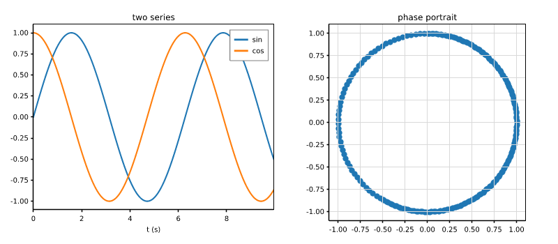
In rizzma panels are subplots, and labels, ticks and the legend follow the
artists:
```rust
# // migrate: panels
use rizzma::Figure;
let cos: Vec<f64> = t.iter().map(|v| v.cos()).collect();
let mut fig = Figure::new(8.0, 3.5);
let ax = fig.add_subplot(1, 2, 1);
ax.plot(&t, &sin).set_label("sin");
ax.plot(&t, &cos).set_label("cos");
ax.set_xlabel("t (s)").set_title("two series");
ax.legend_auto();
let ax = fig.add_subplot(1, 2, 2);
ax.scatter(&sin, &cos);
ax.set_aspect_equal().grid(true);
ax.set_title("phase portrait");
# assert!(!fig.encode_png().unwrap().is_empty());
```
### 2. Images instead of per-pixel loops
```rust,ignore
for (r, row) in data.iter().enumerate() {
for (c, &v) in row.iter().enumerate() {
let color = value_to_color(v, vmin, vmax);
chart.draw_series(std::iter::once(Rectangle::new(
[(c as f64, r as f64), (c as f64 + 1.0, r as f64 + 1.0)], color.filled())))?;
}
}
```
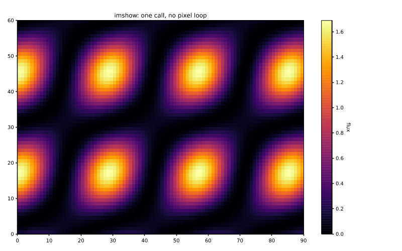
`imshow` takes the row-major values, colormaps and norms them, and a
colorbar reads the same mapping:
```rust
# // migrate: images
use rizzma::Figure;
use rizzma::figure::Mappable;
let (nrows, ncols) = (60, 90);
let data: Vec<f64> = (0..nrows * ncols)
.map(|k| {
let (r, c) = (f64::from(k / ncols) / 9.0, f64::from(k % ncols) / 9.0);
(r.sin() * c.cos() + 0.3 * (r + c).sin()).powi(2)
})
.collect();
let mut fig = Figure::new(8.0, 5.0);
let ax = fig.add_subplot(1, 1, 1);
ax.imshow(&data, nrows as usize, ncols as usize)
.cmap("inferno");
ax.colorbar(Mappable::Image(0)).set_label("flux");
ax.set_title("imshow: one call, no pixel loop");
# assert!(!fig.encode_png().unwrap().is_empty());
```
For cells with explicit edges use `pcolormesh_xy`; for a smooth surface,
`pcolormesh_gouraud`.
### 3. Colormaps instead of copied tables
```rust,ignore
fn value_to_color(v: f64, lo: f64, hi: f64) -> RGBColor {
let t = ((v - lo) / (hi - lo)).clamp(0.0, 1.0);
// 256-entry viridis table pasted from matplotlib...
VIRIDIS[(t * 255.0) as usize]
}
```
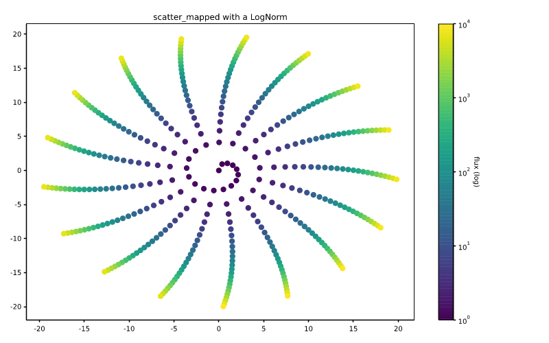
`scatter_mapped` colors points by value through a named colormap and a
norm; `colormap(name)` samples one directly. See
[the colormaps section](#colormaps-the-default-and-what-replaces-jet) for
the default and for replacing jet:
```rust
# // migrate: colormaps
use rizzma::Figure;
use rizzma::core::color::{ColorMapping, LogNorm, colormap};
use rizzma::figure::Mappable;
let n = 400;
let x: Vec<f64> = (0..n)
.map(|i| (f64::from(i) * 0.37).sin() * f64::from(i).sqrt())
.collect();
let y: Vec<f64> = (0..n)
.map(|i| (f64::from(i) * 0.37).cos() * f64::from(i).sqrt())
.collect();
let mut fig = Figure::new(8.0, 5.0);
let ax = fig.add_subplot(1, 1, 1);
ax.scatter_mapped(
&x,
&y,
&flux,
ColorMapping::new("viridis").norm(LogNorm::new(1.0, 1e4)),
);
ax.colorbar(Mappable::Collection(0)).set_label("flux (log)");
ax.set_title("scatter_mapped with a LogNorm");
// One color, for drawing code of your own.
let mid = colormap("viridis").expect("a known colormap").sample(0.5);
assert!(mid.g > mid.r);
# assert!(!fig.encode_png().unwrap().is_empty());
```
### 4. Contours instead of marked cells
```rust,ignore
// "plotters contour support is manual": mark cells near each level
for (i, &v) in grid.iter().enumerate() {
if levels.iter().any(|l| (v - l).abs() < tol) {
chart.draw_series(std::iter::once(Circle::new(cell_center(i), 1, BLACK.filled())))?;
}
}
```
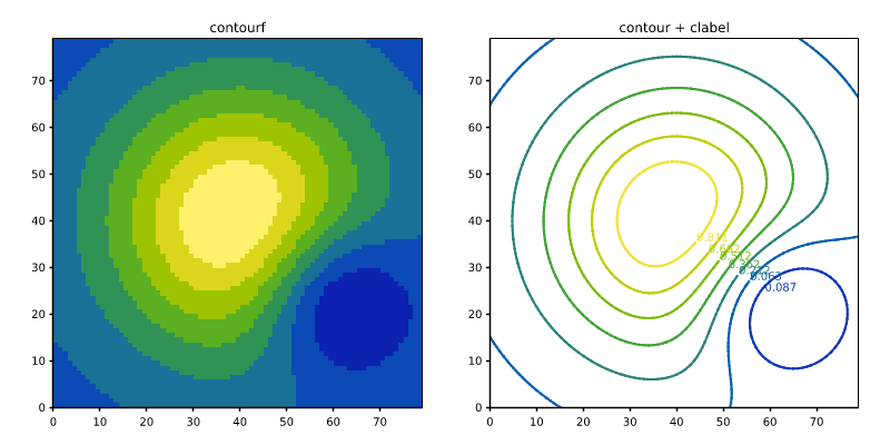
`contourf` fills the bands, `contour` traces the levels by marching
squares, and `clabel` labels them:
```rust
# // migrate: contours
use rizzma::Figure;
let (nrows, ncols) = (80, 80);
let z: Vec<f64> = (0..nrows * ncols)
.map(|k| {
let (x, y) = (
f64::from(k % ncols) / 40.0 - 1.0,
f64::from(k / ncols) / 40.0 - 1.0,
);
(-(x * x + y * y) * 2.0).exp()
- 0.6 * (-((x - 0.5).powi(2) + (y + 0.4).powi(2)) * 6.0).exp()
})
.collect();
let mut fig = Figure::new(8.0, 4.0);
let ax = fig.add_subplot(1, 2, 1);
ax.contourf(&z, nrows as usize, ncols as usize);
ax.set_aspect_equal().set_title("contourf");
let ax = fig.add_subplot(1, 2, 2);
ax.contour(&z, nrows as usize, ncols as usize);
ax.clabel();
ax.set_aspect_equal().set_title("contour + clabel");
# assert!(!fig.encode_png().unwrap().is_empty());
```
### 5. Histograms instead of manual binning
```rust,ignore
let mut counts = vec![0u32; nbins];
for &v in &data {
let b = (((v - lo) / (hi - lo)) * nbins as f64) as usize;
counts[b.min(nbins - 1)] += 1;
}
chart.draw_series(counts.iter().enumerate().map(|(i, &c)| Rectangle::new(
[(bin_left(i), 0.0), (bin_left(i + 1), c as f64)], BLUE.filled())))?;
```
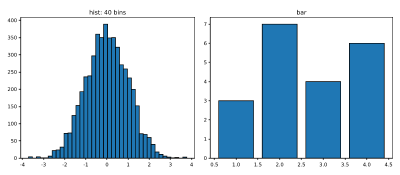
`hist` bins (matplotlib's edges) and draws, and hands back counts and edges;
`bar` draws bars you already have:
```rust
# // migrate: histograms
use rizzma::Figure;
// A deterministic, roughly normal sample: sums of twelve hashed uniforms.
.map(|i| (0..12).map(|k| uniform(i * 12 + k)).sum::<f64>() - 6.0)
.collect();
let mut fig = Figure::new(8.0, 3.5);
let ax = fig.add_subplot(1, 2, 1);
let (counts, edges) = ax.hist(&sample, 40);
assert_eq!((counts.len(), edges.len()), (40, 41));
ax.set_title("hist: 40 bins");
let ax = fig.add_subplot(1, 2, 2);
ax.bar(&[1.0, 2.0, 3.0, 4.0], &[3.0, 7.0, 4.0, 6.0]);
ax.set_title("bar");
# assert!(!fig.encode_png().unwrap().is_empty());
```
### 6. Equal aspect instead of padded ranges
```rust,ignore
// widen whichever range is narrower so circles stay round
let span = (x1 - x0).max(y1 - y0);
let chart = builder.build_cartesian_2d(cx - span / 2.0..cx + span / 2.0,
cy - span / 2.0..cy + span / 2.0)?;
```
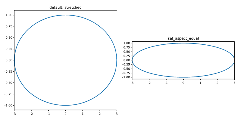
`set_aspect_equal` shrinks the axes box so one data unit is the same length
in x and y, whatever the figure's shape:
```rust
# // migrate: aspect
use rizzma::Figure;
let theta: Vec<f64> = (0..=100)
.map(|i| f64::from(i) * std::f64::consts::TAU / 100.0)
.collect();
let mut fig = Figure::new(8.0, 4.0);
let ax = fig.add_subplot(1, 2, 1);
ax.plot(&x, &y);
ax.set_title("default: stretched");
let ax = fig.add_subplot(1, 2, 2);
ax.plot(&x, &y);
ax.set_aspect_equal().set_title("set_aspect_equal");
# assert!(!fig.encode_png().unwrap().is_empty());
```
### 7. Bands and reference lines instead of hand-built polygons
```rust,ignore
chart.draw_series(std::iter::once(Polygon::new(band, BLUE.mix(0.3))))?;
chart.draw_series(LineSeries::new(vec![(t0, ymin), (t0, ymax)], &RED))?;
```
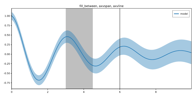
`fill_between`, `axvline` and `axvspan` take data values and span the
current limits for you:
```rust
# // migrate: bands
use rizzma::Figure;
.iter()
.map(|v| (-v / 4.0).exp() * (2.0 * v).cos())
.collect();
let lo: Vec<f64> = model
.iter()
.zip(&t)
.map(|(m, v)| m - 0.1 - 0.02 * v)
.collect();
let hi: Vec<f64> = model
.iter()
.zip(&t)
.map(|(m, v)| m + 0.1 + 0.02 * v)
.collect();
let mut fig = Figure::new(8.0, 4.0);
let ax = fig.add_subplot(1, 1, 1);
ax.fill_between(&t, &lo, &hi);
ax.plot(&t, &model).set_label("model");
ax.axvspan(3.0, 4.5);
ax.axvline(6.0);
ax.legend_auto();
ax.set_title("fill_between, axvspan, axvline");
# assert!(!fig.encode_png().unwrap().is_empty());
```
### 8. Vector fields and secondary axes
```rust,ignore
for (&(x, y), &(u, v)) in points.iter().zip(&vectors) {
chart.draw_series(LineSeries::new(vec![(x, y), (x + u, y + v)], &BLACK))?;
// ...and two more segments for the arrowhead
}
```
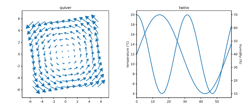
`quiver` draws matplotlib's arrows, scaled together; `twinx` adds an axes
sharing x with its own y scale on the right. Polar plots are a
[`PolarAxes`](crate::figure::PolarAxes) (see
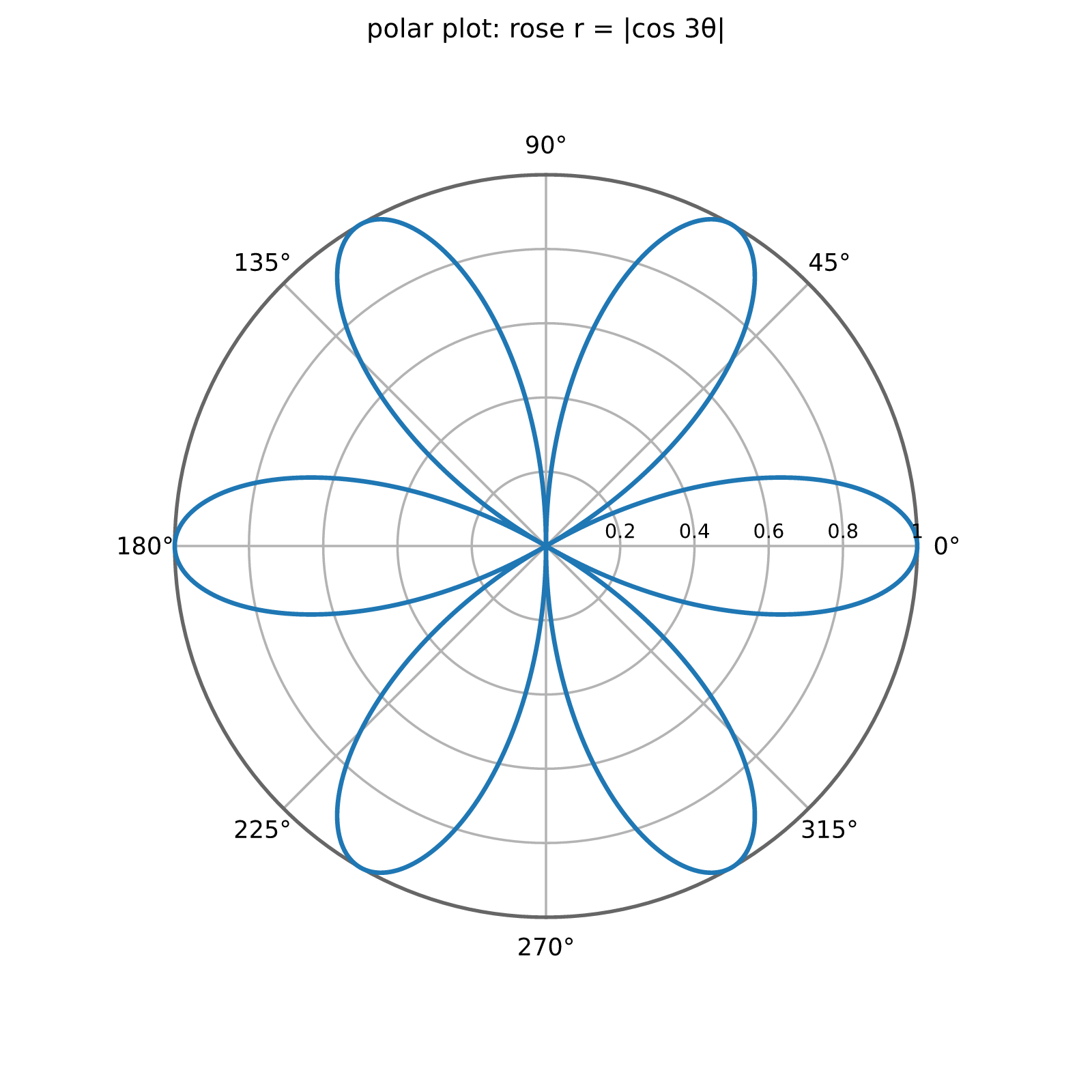).
```rust
# // migrate: vectors
use rizzma::Figure;
let mut x = Vec::new();
let mut y = Vec::new();
for i in 0..12 {
for j in 0..12 {
x.push(f64::from(i) - 5.5);
y.push(f64::from(j) - 5.5);
}
}
let mut fig = Figure::new(8.0, 3.5);
let ax = fig.add_subplot(1, 2, 1);
ax.quiver(&x, &y, &u, &v);
ax.set_aspect_equal().set_title("quiver");
let days: Vec<f64> = (0..60).map(f64::from).collect();
let ax = fig.add_subplot(1, 2, 2);
ax.plot(&days, &temp);
ax.set_ylabel("temperature (°C)").set_title("twinx");
let right = fig.twinx(1);
let twin = &mut fig.axes_mut()[right];
twin.plot(&days, &rain);
twin.set_ylabel("humidity (%)");
# assert!(!fig.encode_png().unwrap().is_empty());
```
### 9. Text without a system font stack
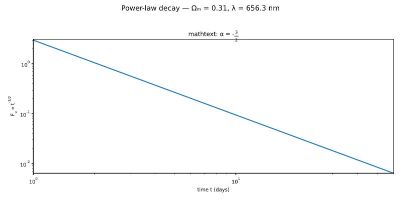
plotters' default build reaches for font-kit, freetype and fontconfig (C
libraries), so projects embed TTFs for `ab_glyph` or hide plotting behind a
feature flag. rizzma embeds DejaVu Sans, the face matplotlib uses, and lays
out text itself, with matplotlib's mathtext for `$…$` spans. Nothing to
install, and the same code renders in wasm:
```rust
# // migrate: text
use rizzma::Figure;
let x: Vec<f64> = (1..=60).map(f64::from).collect();
let mut fig = Figure::new(8.0, 4.0);
fig.suptitle("Power-law decay — Ωₘ = 0.31, λ = 656.3 nm");
let ax = fig.add_subplot(1, 1, 1);
ax.plot(&x, &y);
ax.set_xscale_log(10.0).set_yscale_log(10.0);
ax.set_xlabel(r"time $t$ (days)")
.set_ylabel(r"$F_\nu \propto t^{-3/2}$");
ax.set_title(r"mathtext: $\alpha = -\frac{3}{2}$");
# assert!(!fig.encode_png().unwrap().is_empty());
```
### 10. Bytes and buffers instead of files
```rust,ignore
// plotters only writes files: render to a temp PNG, then read it back
BitMapBackend::new("/tmp/plot.png", (800, 600)).into_drawing_area();
// ...
let bytes = std::fs::read("/tmp/plot.png")?;
```
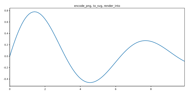
A rizzma figure renders straight to PNG bytes, an SVG string, PDF bytes, or
a pixel buffer you own (a framebuffer, an `image::RgbaImage`, a GUI
texture):
```rust
# // migrate: buffers
use rizzma::Figure;
use rizzma::figure::PixelFormat;
let mut fig = Figure::new(8.0, 4.0);
fig.add_subplot(1, 1, 1).plot(&x, &y);
fig.axes_mut()[0].set_title("encode_png, to_svg, render_into");
let png: Vec<u8> = fig.encode_png().expect("PNG encoding");
let svg: String = fig.to_svg();
let (w, h) = fig.raster_size();
let mut rgba = vec![0u8; w as usize * h as usize * 4];
fig.render_into(&mut rgba, PixelFormat::Rgba8)
.expect("a buffer of the right size");
assert!(png.starts_with(b"\x89PNG") && svg.contains("<svg"));
# assert!(rgba.iter().any(|&b| b != 255));
```
## A worked port: Hipparcos × Gaia magnitudes
OrbitalCommons/starfield's `hipparcos_gaia_match` plots Gaia G against
Hipparcos Hp for cross-matched stars, colored by B−V, with a fitted
relation. Its plotters version (abridged):
```rust,ignore
let root = BitMapBackend::new(out_path, (1200, 900)).into_drawing_area();
root.fill(&WHITE)?;
let (hp_min, hp_max, g_min, g_max, bv_min, bv_max) = data_bounds(data); // 30-line helper
let (g_lo, g_hi) = pad(g_min, g_max);
let mut chart = ChartBuilder::on(&root)
.caption(format!("Hipparcos × Gaia {}: G vs Hp (N={}, RMS={:.3})", rel, data.len(), rms),
("sans-serif", 28))
.margin(20).x_label_area_size(50).y_label_area_size(60)
.build_cartesian_2d(hp_lo..hp_hi, g_lo..g_hi)?;
chart.configure_mesh().x_desc("Hipparcos Hp magnitude")
.y_desc(format!("Gaia {} G magnitude", rel)).draw()?;
chart.draw_series(data.iter().map(|&(hp, bv, g)| {
let t = ((bv - bv_min) / (bv_max - bv_min).max(1e-9)).clamp(0.0, 1.0);
let color = HSLColor(0.7 - 0.7 * t, 0.65, 0.45); // blue → red
Circle::new((hp, g), 2, color.filled())
}))?;
let mean_bv = data.iter().map(|&(_, b, _)| b).sum::<f64>() / data.len() as f64;
let line_pts: Vec<(f64, f64)> = (0..200).map(|i| {
let hp = hp_lo + i as f64 / 199.0 * (hp_hi - hp_lo);
(hp, coef.0 + coef.1 * hp + coef.2 * mean_bv)
}).collect();
chart.draw_series(LineSeries::new(line_pts, BLACK.stroke_width(2)))?
.label(format!("G = {:+.3} {:+.3}·Hp {:+.3}·(B-V) @ <B-V>={:.2}",
coef.0, coef.1, coef.2, mean_bv))
.legend(|(x, y)| PathElement::new(vec![(x, y), (x + 20, y)], BLACK.stroke_width(2)));
chart.configure_series_labels().background_style(WHITE.mix(0.85)).border_style(BLACK).draw()?;
root.present()?;
```
The rizzma port. The bounds helper, padding and label areas go away: limits
autoscale with matplotlib's margins, and the fit line's label feeds the
legend. The hand-made color ramp stays, now as a colormap with a colorbar
that says what it means.
This is a reproduction, not a substitution. `ListedColormap::from_fn` keeps
the original `HSLColor(0.7 − 0.7·t, 0.65, 0.45)` function, plotters' HSL
conversion included, sampled at 256 points like any matplotlib colormap.
At those points its colors equal plotters' exactly. A star between them
takes the nearest entry, within 3 units per channel of plotters' color.
The original's `t` is B−V scaled over the data's range, which is what
`scatter_mapped` does by default. The ramp is still a constant-lightness
rainbow, with the flaws described
[above](#colormaps-the-default-and-what-replaces-jet); for a new figure,
`"coolwarm"` or `"cet_d01"` read blue-to-red without them.
```rust
# // migrate: hipparcos
use rizzma::Figure;
use rizzma::core::color::{ListedColormap, Rgba};
use rizzma::figure::Mappable;
/// starfield's B−V color, plotters' `HSLColor(0.7 − 0.7·t, 0.65, 0.45)`,
/// converted to RGB as plotters does.
fn starfield_bv(t: f64) -> Rgba {
let (h, s, l) = (0.7 - 0.7 * t, 0.65, 0.45);
let q = if l < 0.5 {
l * (1.0 + s)
} else {
l + s - l * s
};
let p = 2.0 * l - q;
let channel = |t: f64| {
let t = t.rem_euclid(1.0);
if t < 1.0 / 6.0 {
p + (q - p) * 6.0 * t
} else if t < 1.0 / 2.0 {
q
} else if t < 2.0 / 3.0 {
p + (q - p) * (2.0 / 3.0 - t) * 6.0
} else {
p
}
};
Rgba::rgb(channel(h + 1.0 / 3.0), channel(h), channel(h - 1.0 / 3.0))
}
/// G against Hp, colored by B−V, with the fitted relation at the mean B−V.
fn plot_g_vs_hp(data: &[(f64, f64, f64)], coef: (f64, f64, f64), rms: f64) -> Figure {
let hp: Vec<f64> = data.iter().map(|d| d.0).collect();
let bv: Vec<f64> = data.iter().map(|d| d.1).collect();
let g: Vec<f64> = data.iter().map(|d| d.2).collect();
let mean_bv = bv.iter().sum::<f64>() / bv.len() as f64;
let (lo, hi) = hp
.iter()
.fold((f64::INFINITY, f64::NEG_INFINITY), |(lo, hi), &v| {
(lo.min(v), hi.max(v))
});
let fit_hp = [lo, hi];
let fit_g = fit_hp.map(|h| coef.0 + coef.1 * h + coef.2 * mean_bv);
let mut fig = Figure::new(8.0, 6.0);
let ax = fig.add_subplot(1, 1, 1);
ax.scatter_mapped(&hp, &g, &bv, ListedColormap::from_fn(starfield_bv))
.set_sizes(vec![4.0]);
ax.plot(&fit_hp, &fit_g)
.set_linewidth(2.0)
.set_label(format!(
"G = {:+.3} {:+.3}·Hp {:+.3}·(B−V) at ⟨B−V⟩ = {mean_bv:.2}",
coef.0, coef.1, coef.2
));
ax.colorbar(Mappable::Collection(0)).set_label("B − V");
ax.legend_auto();
ax.set_xlabel("Hipparcos Hp magnitude")
.set_ylabel("Gaia DR3 G magnitude");
ax.set_title(format!(
"Hipparcos × Gaia DR3: G vs Hp (N={}, RMS={rms:.3})",
data.len()
));
fig
}
// Synthetic stand-in for the cross-match: G ≈ Hp − 0.2 − 0.3·(B−V).
let data: Vec<(f64, f64, f64)> = (0..1500)
.map(|i| {
let u = (f64::from(i) * 0.618_034).fract();
let w = (f64::from(i) * 0.414_214).fract();
let hp = 2.0 + 8.0 * u.sqrt();
let bv = -0.2 + 1.8 * w;
(
hp,
bv,
hp - 0.2 - 0.3 * bv + 0.05 * (f64::from(i) * 1.7).sin(),
)
})
.collect();
let fig = plot_g_vs_hp(&data, (-0.2, 1.0, -0.3), 0.035);
# assert!(!fig.encode_png().unwrap().is_empty());
# // The ramp matches plotters at the ends and the middle (the full check is
# // tests/custom_colormaps.rs).
# assert_eq!(starfield_bv(0.0).to_u8_array(), [70, 40, 189, 255]);
# assert_eq!(starfield_bv(127.0 / 255.0).to_u8_array(), [40, 189, 56, 255]);
# assert_eq!(starfield_bv(1.0).to_u8_array(), [189, 40, 40, 255]);
```
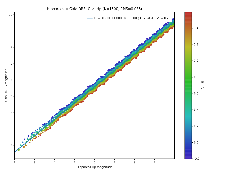
To write it, `fig.save_png(out_path)?` replaces `root.present()`, and a
`PngError` replaces the `plotter_err` mapping helper.