gravimetry

Satellite gravimetry from instrument to map. Model the satellites, from today's GRACE-FO to missions with quantum (cold-atom) sensors, and simulate what gravity field they recover. Then turn the monthly fields of GRACE and GRACE-FO into maps of water storage, and model the gravity change an earthquake causes. Built on geopotential.

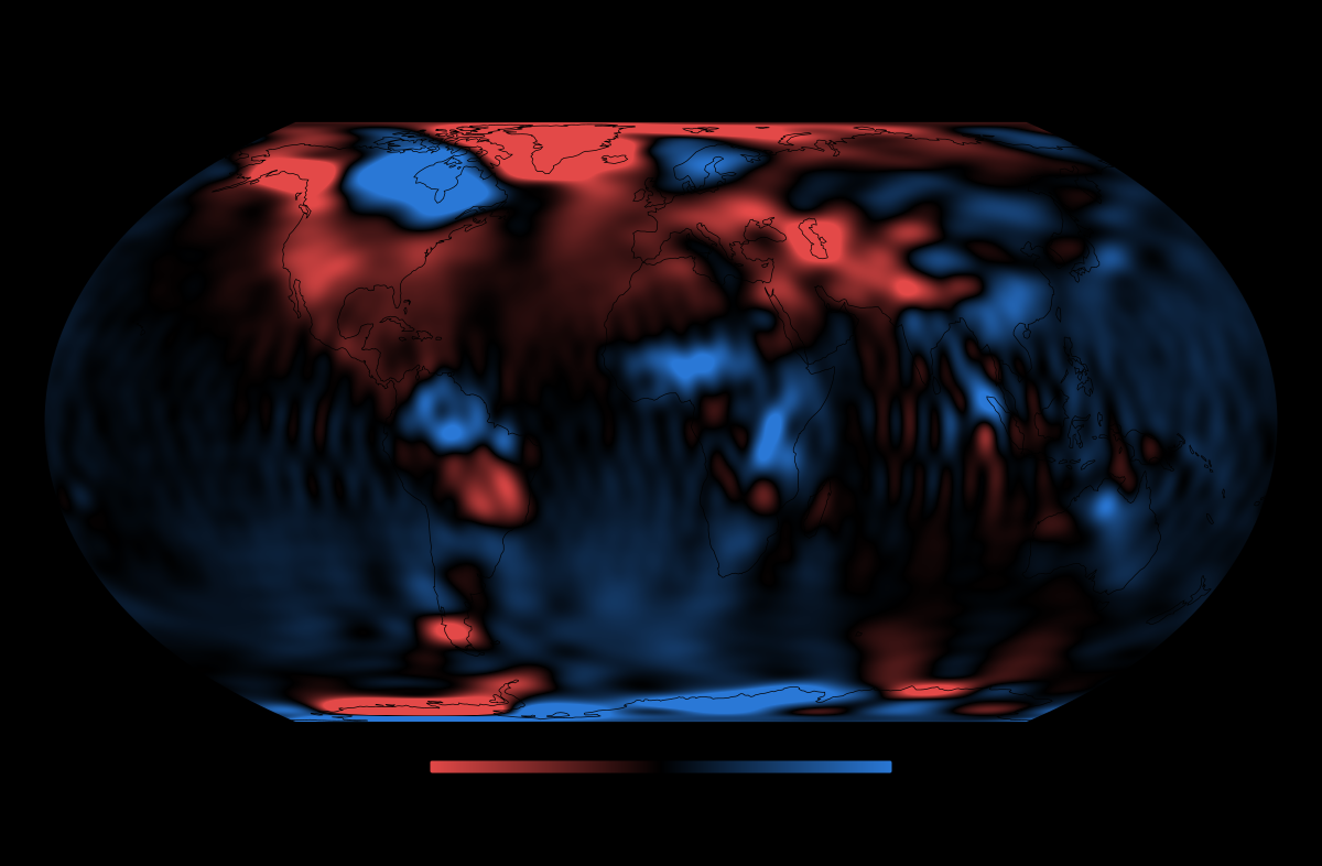
Water stored on land and in the ocean in July 2026, against the 2004–2009 average.

Install

cargo add gravimetry geopotential

Example: from a monthly field to water height

The standard chain of the GRACE Tellus maps (Landerer & Swenson 2012):

1. subtract a baseline;
2. remove the stripes;
3. smooth over 300 km;
4. convert to centimetres of water.

use geopotential::{Coefficients, Functional};

let (gm, radius) = (3.986004415e14, 6_378_136.3);

// A month and the baseline it is compared with (here: one changed coefficient).
let mut month = Coefficients::zeros(gm, radius, 60);
month.set(2, 0, 1e-10, 0.0);
let baseline = Coefficients::zeros(gm, radius, 60);

let change = gravimetry::anomaly(&month, &baseline);
let change = gravimetry::destripe(&change);
let change = gravimetry::smooth(&change, &gravimetry::gaussian_weights(300e3, radius, 60));

let love = gravimetry::love_numbers(60).unwrap();
let water = change.grid(&Functional::WaterHeight { love: &love }, radius, &[90f64.to_radians()], &[0.0]);
println!("{:.0} mm of water at the North Pole", water[0] * 1000.0); // 19 mm

With real data, read each month with geopotential::read_gfc and the low-degree corrections with technotes::read_tn14 and read_tn13. The full chain replaces C̄20, C̄30 and degree 1 before subtracting the baseline.

Example: a quantum accelerometer against GRACE-FO

Instrument noise, reproducing Figure 1 of Zingerle et al. (2024) from its equations.

use gravimetry::atom::AtomInterferometer;
use gravimetry::missions::{Accelerometer, Ranging, pair_noise};

// A cold-atom accelerometer like CARIOQA's: 1 s between pulses, 80% contrast,
// 100,000 atoms per shot, one shot every 3.5 s, double diffraction in orbit.
let atoms = AtomInterferometer { t: 1.0, contrast: 0.8, atoms: 1e5, cycle: 3.5, diffraction: 2 };
let white = atoms.acceleration_asd(); // about 2.3e-10 m/s² per √Hz

// Noise of a satellite pair at 0.1 mHz, the longest wavelengths, in m/s² per √Hz.
let quantum = pair_noise(Accelerometer::AtomInterferometer { white }, Ranging::Lri2033, 1e-4);
let today = pair_noise(Accelerometer::SuperStar, Ranging::GraceFo, 1e-4);
println!("quantum {quantum:.1e}, GRACE-FO {today:.1e}"); // 3.2e-10 against 1.0e-9
assert!(quantum < today / 3.0);

Example: the gravity change of an earthquake

Left: the gravity step the July 2025 Kamchatka earthquake left in GRACE-FO. Right: the USGS fault model through the same filter, computed with this crate.

use gravimetry::coseismic::{Fault, Medium};

// A thrust fault: 100 × 50 km, 8 m of slip, its centre 20 km deep.
let fault = Fault {
    lat: 52.5, lon: 160.0, depth: 20e3,
    strike: 217.0, dip: 15.0, rake: 90.0,
    length: 100e3, width: 50e3, slip: 8.0, opening: 0.0,
};

// Uplift and gravity change at the surface straight above it.
let above = fault.surface_change(0.0, 0.0, &Medium::default());
println!("uplift {:.2} m, gravity {:+.0} µGal", above.uplift, above.gravity * 1e8); // 1.20 m, +115 µGal

// What a satellite sees: surface masses on a grid, as coefficients, smoothed like the data.
let lats: Vec<f64> = (0..50).map(|i| (47.0 + 0.2 * i as f64).to_radians()).collect();
let lons: Vec<f64> = (0..70).map(|j| (153.0 + 0.2 * j as f64).to_radians()).collect();
let at_sea = |_lat: f64, _lon: f64| true;
let masses = gravimetry::coseismic::surface_masses(&[fault], &lats, &lons, &Medium::default(), at_sea);
let field = gravimetry::mass_coefficients(&masses, 3.986004415e14, 6_378_136.3, 60);
let field = gravimetry::smooth(&field, &gravimetry::gaussian_weights(300e3, field.radius, 60));

For a real earthquake, coseismic::read_coulomb reads the coulomb.inp file that the USGS publishes with every finite-fault model.

Example: fill the gaps in a monthly record

The GRACE record has gaps: missing months, and almost a year between the two missions. The Kalman smoother treats each coefficient as a slowly wandering signal plus noise. It gives the best estimate and its uncertainty for every month, gaps included.

use gravimetry::kalman::{Process, smooth};

// Five months, the middle one missing, each observed with an error of 1.
let times = [0.0, 1.0, 2.0, 3.0, 4.0].map(|month| month / 12.0);
let observed = [Some((1.0, 1.0)), Some((2.0, 1.0)), None, Some((2.5, 1.0)), Some((2.0, 1.0))];

// A signal that varies by about 2 over about 6 months.
let result = smooth(&times, &observed, Process { sd: 2.0, tau: 0.5 });
println!("month 3: {:.2} ± {:.2}", result.mean[2], result.sd[2]);

kalman::fit picks the signal's size and correlation time, and checks the stated errors, by maximum likelihood over many series at once.

What is inside

The simulated error of four mission classes, from today's to a quantum pair, against the errors of a real month.

Applications

• Drought and groundwater. GRACE and GRACE-FO mass change feeds weekly drought indicators and statutory groundwater reporting; the processing chain here is the one those products use.
• Ice sheets and sea level. examples/ice_and_sea_level.rs turns Greenland's published mass trend into its sea-level contribution.
• Earthquakes. coseismic models the gravity change of a fault and reads USGS finite-fault files; prompt_lead gives how far ahead of the P-wave a light-speed gravity signal arrives.
• Site surveys and monitoring. local gives the gravity and gradient of a buried void or dense body, and the averaging time a quantum gravimeter needs to resolve it.
• Absolute gravimetry. tides corrects a reading for the lunar and solar tide and moves it between the zero-tide convention of gravity and the mean-tide convention of the IHRS.
• Mission design. missions, atom and sim size the sensors and simulate what field a satellite pair recovers, including cold-atom instruments.

How it is checked

• Noise models: they reproduce Figure 1 of Zingerle et al. (2024).
• Cold-atom sensors: they reproduce the published CARIOQA, GRICE and Trimeche et al. (2019) sensitivities.
• Gradiometry errors: the closed form matches brute-force least squares.
• Simulator: it recovers a known field exactly without noise; with noise, a χ² test confirms that its actual errors match its predicted ones.
• Technical notes: real NASA files, excerpted in tests/data.
• Love numbers: against the published table. Smoothing weights: against their closed-form limit. Stripe removal: on synthetic patterns.
• Fault model: Okada's (1985) published check values; mass conservation (a buried fault's equivalent mass sums to zero); on the 2025 Kamchatka fault model, its uplift matches the USGS's own surface displacement with r = 0.89.
• Point masses: their potential matches Newton's law.
• Tides: LongmanTide's test vector to 3×10⁻¹¹ mGal; averaged over the 18.61-year nodal cycle, Longman's tide is δ₂ times the permanent tide to 0.2 µGal; the permanent tide matches Mäkinen's (2021) Eqs. 19–21 to their printed digits.
• Kalman smoother: it matches the exact Gaussian-process solution to 1e-10, its fit recovers the settings of simulated data, and on the real record withheld months are predicted with calibrated errors.
• Atmosphere: the isothermal values at 250 K (sound 317 m/s, cut-off 0.0217 rad/s, buoyancy 0.0196 rad/s); the Lamb wave is trapped at every wavelength; the Tonga Lamb speed of 318.2 m/s is sound at 252 K; a slow pressure pulse gives the inverse barometer.

Not included yet: glacial isostatic adjustment, DDK filters, basin averages and leakage corrections; time-variable gravity in the simulator, so no temporal aliasing.

One of eight crates in physica: physica (all of them, plus cross-domain analogies) · metrology (constants) · geopotential (the gravity field) · gravimetry (missions and GRACE) · gravitational (waves) · gravitics (frontier gravity) · magnetics (magnetism and MHD) · plasmoid (fusion plasma).