# Tests
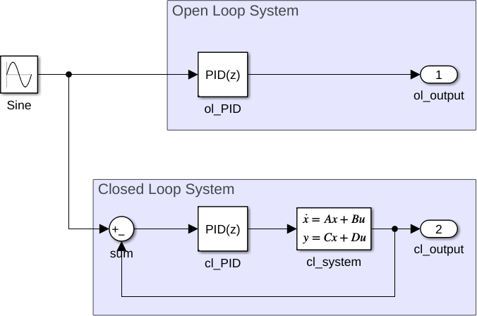
Our crate's crucial advantage is that our PID controller is tested against the
Simulink **PID Controller Block** in both open-loop and closed-loop simulations.
In the open-loop case, the PID controller is simply given a sine-wave setpoint
while the process value is fixed at 0.
In the closed-loop case, the PID controller is used to drive a
mass-spring-damper system to track a sine references.
```math
\ddot{x} + 2\zeta\omega_n^2\dot{x} + x = u
```
In both cases, the PID controller is configured with non-default parameters.
## Recreating the test data
The test data is generated by `generate_test_data.m`. If you have a MATLAB
installation, you can directly run this script.
This script does the following:
1. Create a temporary Simulink model programmatically
2. Define the Simulink blocks and topology
3. Simulates the model
4. Writes the simulation output to a rust source file
## Recreating the Model
The models are configured as shown below
The configuration parameters of the models can be retrieved from
`generate_test_data.m`, but they are repeated here for your convenience
| Model Settings - Solver | Solver Type | ODE1 (Euler) |
| Model Settings - Solver | Fixed Stepsize | 0.01 |
| Model Settings - Data Export | Format | Array |
| PID | P | 10.0 |
| PID | I | 20.0 |
| PID | D | 1.0 |
| PID | Filter Coefficient/N | 50 |
| State-Space | A | See below |
| State-Space | b | See Below |
| State-Space | c | `[1, 0]` |
| State-Space | d | `0` |
The `A` and `b` matrices of the state-space model are given by
```math
\mathbf{A} = \begin{bmatrix}
0 & 1 \\
-2\zeta\omega_n & -\omega_n^2
\end{bmatrix} \quad
\mathbf{b} = \begin{bmatrix}
0 \\ \omega_n^2
\end{bmatrix}
```
Where the damping ratio ζ is set to 0.2, and the natural frequency ωₙ is set to
2π.