# SLAM Path Optimization
Arael's SLAM example is a visual-inertial backend: it jointly optimises
robot poses and landmark positions from camera observations, GPS,
wheel odometry, and accelerometer tilt readings. The focus is on the
numerical backend -- nonlinear least squares with symbolic
differentiation. Landmark discovery, feature detection, and data
association are out of scope and are supplied as synthetic data.
The demo generates a synthetic S-curve trajectory with 60 poses and
240 point landmarks at 5-30m distance. Five cameras provide
360-degree coverage. Each landmark is visible from its anchor pose
+/- 15 poses with 75% probability, reproducing the sparse band
structure you get from real feature tracks. **50% of feature
associations are completely wrong, with 30x pixel noise on those
outliers** -- tolerated by the Starship robust wrapper combined with
graduated optimisation.
The linear solver is faer sparse Cholesky (pure Rust) to exploit the
Hessian sparsity, with optional Eigen SimplicialLLT and CHOLMOD
backends via C++ FFI. On the default problem size (200 poses) the
sparse path is 66x faster than dense. Problem size and solver are
command-line flags:
```bash
cargo run -r --example slam_demo -- --solver faer --poses 100 --landmarks 400
```
## Problem structure
Each entity owns its own parameters and its own `SelfBlock` -- the
diagonal block of the Hessian for that entity. Constraints that
touch a single entity accumulate into its self block; constraints
that couple two entities (odometry between two poses, a bearing
residual between a landmark and a pose) accumulate into a
`CrossBlock` between the pair. The assembled Hessian mirrors the
model hierarchy: one block row/column per entity, a self block on
the diagonal, and a cross block off-diagonal wherever a constraint
ties two entities together. Entities that never share a constraint
remain exactly zero in that corner of the matrix -- that is where
the sparsity comes from.
```
Path (root)
poses: Deque<Pose> -- 60 poses, 6 params each (pos + ea)
pos: Param<vect3f> -- 3D position (optimizable)
ea: SimpleEulerAngleParam<f32> -- euler angles: x=roll, y=pitch, z=yaw
info: PoseInfo -- odometry, GPS, tilt, features
hb_pose: SelfBlock<Pose> -- GPS + drift + tilt hessian block
landmarks: Vec<PointLandmark> -- 240 landmarks, 3 params each
pos: Param<vect3f> -- 3D position (optimizable)
frines: Vec<PointFrine> -- observations linking to poses
pose: Ref<Pose> -- which pose observed this
feature: Ref<PointFeature> -- feature data
hb: CrossBlock<PointLandmark, Pose>
hb_drift: SelfBlock<PointLandmark> -- landmark drift regularizer
pose_pairs: Vec<PosePair> -- 59 consecutive pose pairs
prev: Ref<Pose> -- previous pose
cur: Ref<Pose> -- current pose
hb: CrossBlock<Pose, Pose> -- odometry hessian block
gamma: f32 -- Starship suppression parameter
drift_pos_isigma: f32 -- pose position drift (1/1000m)
drift_ea_isigma: f32 -- pose ea drift (1/deg2rad(1800))
drift_lm_isigma: f32 -- landmark drift (1/1000m)
tilt_isigma: f32 -- tilt sensor (1/deg2rad(0.25))
```
Total: 1080 parameters (60 * 6 + 240 * 3). Configurable via `--poses`
and `--landmarks`.
### Frines
A **frine** (project vocabulary) is a struct that ties one entity to
one measurement. `PointFrine` is the frine for a point landmark: it
binds a `PointLandmark` to a `PointFeature` -- the 2D detection in
one of the pose's cameras that observed it. In factor-graph SLAM
terms a frine is what GTSAM calls a `Factor` and g2o an `Edge`.
The measurement is pre-processed once at set-up time into a 3D
direction ray in the camera frame (stored on `PointFeature`), so the
solver never touches pixel coordinates or undistortion. Staying in
3D keeps derivatives smooth and sidesteps the projective
singularities that appear when you differentiate through a
pixel-space reprojection.
## Hessian sparsity

The sparsity pattern shows pose-pose blocks in the upper-left
(odometry coupling consecutive poses), pose-landmark coupling in the
off-diagonal rectangles (each landmark visible from nearby poses
only), and landmark self-blocks along the lower-right diagonal.
Sorting landmarks by anchor pose would produce an arrowhead pattern;
here they are in insertion order. Sparse Cholesky exploits this
structure for large speedups over dense solvers.
## Gauge freedom
Without absolute reference, visual SLAM has 6 degrees of gauge
freedom (3 translation + 3 rotation). The entire solution can
shift/rotate arbitrarily without changing feature reprojection costs.
Each sensor fixes specific degrees of freedom:
- **Tilt sensor (accelerometer)** fixes roll (ea.x) and pitch (ea.y),
making the path level. Without it the solution can tilt arbitrarily.
- **GPS** fixes translation and yaw (ea.z). Even with a systematic
offset (all readings biased by ~2.5m), it still constrains yaw
because the offset is constant while poses move -- relative GPS
positions define heading.
- **Odometry** constrains relative motion between consecutive poses.
- **Drift constraints** are weak regularizers (sigma=1000m pos,
1800deg ea) preventing parameters from diverging during early
optimization passes when feature constraints are scaled down.
## Entities
Every struct in the model hierarchy is shown here with its fields and
every constraint attached to it. Read top-down: each entity is
introduced, then its fields, then (if it carries any) the constraints
that contribute to the assembled Hessian. The model is
`#[arael::model]`-annotated throughout; the macros walk this entire
hierarchy from `Path` downward and emit one fused `calc_cost` /
`calc_grad_hessian` pair.
### `PointFeature` -- a single camera detection
A `PointFeature` is the pre-processed form of one 2D feature
detection in one of a pose's cameras. Pre-processing happens once at
set-up time; from then on the solver reasons about direction rays in
3D, never about pixel coordinates.
```rust
#[arael::model]
#[allow(dead_code)]
struct PointFeature {
pixel: vect2f,
mf2r: matrix3f, // feature-to-robot rotation: col0=view dir, col1/col2=perp axes
#[arael(skip)]
camera: Ref<Camera>,
camera_pos: vect3f, // camera position in robot frame
isigma: vect2f, // 1/sigma for angular residuals (rad^-1)
}
```
- `pixel` -- the original detection pixel; kept for debugging, not
touched by any constraint.
- `mf2r` -- the **feature frame** rotation. `col0` points from the
pose along the measured view direction (in robot-frame
coordinates); `col1` and `col2` are the two perpendicular axes
used to measure horizontal and vertical angular error. Set at
observation time from the pixel's ray and the camera extrinsics.
- `camera` -- handle to the `Camera` that saw the feature. The
`#[arael(skip)]` annotation tells the macro to ignore this field
when computing `PARAM_COUNT`; the solver never differentiates
through `Camera`, it only needs `camera_pos` and `mf2r`.
- `camera_pos` -- the camera's position in the robot's body frame.
- `isigma` -- `1/sigma_x` and `1/sigma_y` for the two angular
residuals, expressed in `rad^-1`. Usually comes from the pixel
noise divided by `fx` / `fy`.
`PointFeature` carries no constraints of its own; it is pure
measurement data. The constraint that uses it lives on `PointFrine`.
### `GpsData` -- a decomposed GPS reading
```rust
#[arael::model]
struct GpsData {
pos: vect3f,
cov_r: matrix3f,
cov_isigma: vect3f,
}
```
- `pos` -- the GPS position reading in world frame.
- `cov_r` / `cov_isigma` -- eigendecomposition of the covariance
`K = R * diag(d) * R^T`, stored as `R` and `1/sqrt(d)`. Whitening
a raw difference `raw = pose.pos - gps.pos` is then just
`whitened = diag(cov_isigma) * cov_r^T * raw`, which makes the
residual a plain sigma count and gives Gauss-Newton a spherical
local geometry. The decomposition is done once at set-up time by
the helper below:
```rust
fn decompose_cov(cov: matrix3f) -> (matrix3f, vect3f) {
let (r, d) = cov.symmetric_eigen();
let isigma = vect3f::new(
1.0 / d.x.sqrt(), 1.0 / d.y.sqrt(), 1.0 / d.z.sqrt());
(r, isigma)
}
```
`GpsData` has no constraints -- it is held by `PoseInfo` as
`Option<GpsData>` and consumed by the guarded GPS constraint on
`Pose`.
### `PoseInfo` -- all per-timestep measurements on one Pose
```rust
#[arael::model]
struct PoseInfo {
delta_pos: vect3f,
delta_ea: vect3f,
delta_pos_cov_r: matrix3f,
delta_pos_cov_isigma: vect3f,
delta_ea_cov_r: matrix3f,
delta_ea_cov_isigma: vect3f,
gps: Option<GpsData>,
tilt_roll: f32,
tilt_pitch: f32,
features: refs::Vec<PointFeature>,
}
```
- `delta_pos`, `delta_ea` -- wheel-odometry measurement of the
motion from the *previous* pose to this one, expressed in the
previous pose's frame.
- `delta_pos_cov_r` / `delta_pos_cov_isigma`,
`delta_ea_cov_r` / `delta_ea_cov_isigma` -- decomposed odometry
covariances, produced by `decompose_cov` on the position and
attitude covariances separately.
- `gps: Option<GpsData>` -- optional GPS fix at this timestep. The
GPS constraint on `Pose` is **guarded** on `self.info.gps.is_some()`
so the macro emits a conditional that evaluates the constraint
only where a fix actually exists.
- `tilt_roll`, `tilt_pitch` -- accelerometer readings projected into
roll (ea.x) and pitch (ea.y) at this timestep.
- `features: refs::Vec<PointFeature>` -- the list of point features
detected from this pose. Each entry is the set-up-time result of
matching a 2D detection to a camera and pre-computing its
`mf2r` / `camera_pos` / `isigma`.
`PoseInfo` has no constraints on itself either -- it is the
data side-car consumed by constraints on `Pose` and `PointFrine`.
### `Pose` -- the optimised 6-DOF state
This is where three constraints stack. All three accumulate into the
same `hb_pose: SelfBlock<Pose>`.
```rust
#[arael::model]
#[arael(constraint(hb_pose, guard = self.info.gps.is_some(), {
let gamma = path.gamma;
let raw = pose.pos - pose.info.gps.pos;
let rt_raw = pose.info.gps.cov_r.transpose() * raw;
let p0 = rt_raw.x * pose.info.gps.cov_isigma.x;
let p1 = rt_raw.y * pose.info.gps.cov_isigma.y;
let p2 = rt_raw.z * pose.info.gps.cov_isigma.z;
[gamma * atan(p0 / gamma),
gamma * atan(p1 / gamma),
gamma * atan(p2 / gamma)]
}))]
#[arael(constraint(hb_pose, {
let pos_drift = pose.pos - pose.pos_value;
let ea_drift = pose.ea - pose.ea_value;
[pos_drift.x * path.drift_pos_isigma,
pos_drift.y * path.drift_pos_isigma,
pos_drift.z * path.drift_pos_isigma,
ea_drift.x * path.drift_ea_isigma,
ea_drift.y * path.drift_ea_isigma,
ea_drift.z * path.drift_ea_isigma]
}))]
#[arael(constraint(hb_pose, {
[(pose.ea.x - pose.info.tilt_roll) * path.tilt_isigma,
(pose.ea.y - pose.info.tilt_pitch) * path.tilt_isigma]
}))]
struct Pose {
pos: Param<vect3f>,
ea: SimpleEulerAngleParam<f32>,
info: PoseInfo,
hb_pose: SelfBlock<Pose>,
}
```
Fields:
- `pos: Param<vect3f>` -- the pose's 3D position. `Param<T>` marks
this as an **optimisation variable**; the macro counts 3 scalars
into `PARAM_COUNT` for `Pose` and threads their indices through
`calc_grad_hessian`.
- `ea: SimpleEulerAngleParam<f32>` -- the pose's orientation as
Euler angles `(roll=x, pitch=y, yaw=z)`, another 3 scalars.
`SimpleEulerAngleParam` precomputes `sin`/`cos` of the three
angles and the `3x3` rotation matrix in the update cycle, so
constraint bodies can call `pose.ea.rotation_matrix()` without the
trig appearing in the differentiated code.
- `info: PoseInfo` -- all per-timestep measurements (above). Not
optimised, just read.
- `hb_pose: SelfBlock<Pose>` -- the Hessian block covering this
pose's own 6 parameters. All three constraints below write into
this same block.
Constraints:
1. **GPS, guarded** (first attribute). Whitened position residual
wrapped by Starship. `guard = self.info.gps.is_some()` tells the
macro to only evaluate when this particular pose actually has a
GPS fix -- there is no `else` branch, no wasted work, no NaN
hazard. The covariance is decomposed into `cov_r` (rotation to
principal axes) and `cov_isigma` (`1/sigma` along each axis);
applying `cov_r^T * raw` and scaling by `cov_isigma` is the
whitening `diag(1/sqrt(d)) * R^T * (pose.pos - gps.pos)`.
2. **Drift regularizer** (second attribute). The macro generates
shadow fields `pose.pos_value` and `pose.ea_value` from every
`Param<...>` field -- they hold the parameter's initial value.
The residual measures drift away from that anchor and weights it
by a very loose sigma (drift_pos = 1000m, drift_ea = 1800deg in
the demo). The only purpose is to keep the early passes, where
feature constraints are scaled down, from wandering off into
regions where GPS and odometry no longer pull hard enough.
3. **Tilt** (third attribute). Directly constrains roll and pitch to
the accelerometer readings on this timestep. This is what fixes
the two rotational gauge DOFs that GPS alone cannot pin down.
### `PointLandmark` -- the 3D landmark entity
```rust
#[arael::model]
#[arael(constraint(hb_drift, {
let drift = pointlandmark.pos - pointlandmark.pos_value;
[drift.x * path.drift_lm_isigma,
drift.y * path.drift_lm_isigma,
drift.z * path.drift_lm_isigma]
}))]
struct PointLandmark {
pos: Param<vect3f>,
frines: std::vec::Vec<PointFrine>,
hb_drift: SelfBlock<PointLandmark>,
}
```
Fields:
- `pos: Param<vect3f>` -- 3 scalars, the optimised landmark
position.
- `frines: std::vec::Vec<PointFrine>` -- the observations that tie
this landmark to poses. Owned by the landmark so the macro walks
them when generating feature constraints; one landmark typically
has many frines.
- `hb_drift: SelfBlock<PointLandmark>` -- this landmark's diagonal
Hessian block.
Constraint:
- **Landmark drift regularizer.** Same idea as the pose drift above
but on the landmark position: anchor to the initial `pos_value`
with a very weak sigma (`drift_lm_isigma = 1/1000m`). The
bare-name `pointlandmark` in the body is the default -- when
`parent` is not specified, the macro uses the struct name
lowercased. So `pointlandmark.pos_value` refers to this
landmark's set-up-time position.
Feature observations live on `PointFrine`, not here, because they
couple a landmark to a pose and need a `CrossBlock` spanning both.
### `PointFrine` -- the landmark-to-pose observation
A **frine** (project vocabulary) is a struct that ties one entity to
one measurement. `PointFrine` is the frine for a point landmark: it
binds a `PointLandmark` to a `PointFeature`. In factor-graph SLAM
terms a frine plays the role of a `Factor` (GTSAM) or an `Edge`
(g2o).
```rust
#[arael::model]
#[arael(constraint(hb, parent=lm, {
let gamma = path.gamma;
let mr2w = pose.ea.rotation_matrix();
let lm_r = mr2w.transpose() * (lm.pos - pose.pos);
let r_r = lm_r - feature.camera_pos;
let r_f = feature.mf2r.transpose() * r_r;
let plain1 = atan2(r_f.y, r_f.x) * feature.isigma.x * path.frine_isigma_scale;
let plain2 = atan2(r_f.z, r_f.x) * feature.isigma.y * path.frine_isigma_scale;
let err1 = gamma * atan(plain1 / gamma);
let err2 = gamma * atan(plain2 / gamma);
[err1, err2]
}))]
struct PointFrine {
#[arael(ref = root.poses)]
pose: Ref<Pose>,
#[arael(ref = pose.info.features)]
feature: Ref<PointFeature>,
hb: CrossBlock<PointLandmark, Pose>,
}
```
Fields:
- `pose: Ref<Pose>` with `#[arael(ref = root.poses)]` -- the
observing pose, resolved from the root's `poses` collection.
- `feature: Ref<PointFeature>` with
`#[arael(ref = pose.info.features)]` -- **chained resolution**.
The `pose` reference has just been resolved; the macro now looks
the feature up inside *that pose's* `info.features`. Chained
refs let you model "this observation in that pose's camera"
without duplicating camera / feature data on the frine.
- `hb: CrossBlock<PointLandmark, Pose>` -- cross-Hessian block
spanning the landmark's 3 params and the pose's 6 params.
Constraint:
- **Bearing observation.** `parent=lm` tells the macro to expose the
parent `PointLandmark` variable as `lm` in the body (since the
frine lives inside a landmark via `PointLandmark::frines`). Steps:
1. Landmark into robot frame: `lm_r = R^T * (lm.pos - pose.pos)`.
2. Subtract camera offset: `r_r = lm_r - feature.camera_pos`.
3. Transform to feature frame:
`r_f = feature.mf2r^T * r_r`.
4. Two angular residuals: `atan2(r_f.y, r_f.x)` (horizontal) and
`atan2(r_f.z, r_f.x)` (vertical). Using `atan2` on the
landmark direction keeps the derivatives smooth and avoids the
projective singularities of a pixel-space reprojection.
5. Whiten by the feature's per-axis `isigma`, then multiply by
the global `frine_isigma_scale` so **graduated optimisation**
can dial all feature constraints up or down as a group from
the root.
6. Starship cap: `gamma * atan(plain / gamma)` on each.
Because the `CrossBlock<PointLandmark, Pose>` names both parents,
the macro knows the Jacobian row writes into both the landmark's
and the pose's diagonal blocks on the self-block side, and into
the cross block on the off-diagonal.
### `PosePair` -- the odometry edge
```rust
#[arael::model]
#[arael(constraint(hb, {
let mr2w_prev = prev.ea.rotation_matrix();
let pos_diff = mr2w_prev.transpose() * (cur.pos - prev.pos);
let pos_err = pos_diff - cur.info.delta_pos;
let pos_w = cur.info.delta_pos_cov_r.transpose() * pos_err;
let mr2w_cur = cur.ea.rotation_matrix();
let expected = mr2w_prev * cur.info.delta_ea.rotation_matrix();
let error_rot = expected.transpose() * mr2w_cur;
let ea_err = error_rot.get_euler_angles();
let ea_w = cur.info.delta_ea_cov_r.transpose() * ea_err;
[pos_w.x * cur.info.delta_pos_cov_isigma.x,
pos_w.y * cur.info.delta_pos_cov_isigma.y,
pos_w.z * cur.info.delta_pos_cov_isigma.z,
ea_w.x * cur.info.delta_ea_cov_isigma.x,
ea_w.y * cur.info.delta_ea_cov_isigma.y,
ea_w.z * cur.info.delta_ea_cov_isigma.z]
}))]
struct PosePair {
#[arael(ref = root.poses)]
prev: Ref<Pose>,
#[arael(ref = root.poses)]
cur: Ref<Pose>,
hb: CrossBlock<Pose, Pose>,
}
```
Fields:
- `prev: Ref<Pose>` and `cur: Ref<Pose>` -- the two consecutive
poses. Both resolve against `root.poses`.
- `hb: CrossBlock<Pose, Pose>` -- the off-diagonal block coupling
the two poses' 6-param blocks. Each `PosePair` contributes one
such 6x6 block on the pose-pose band.
Constraint:
- **Relative motion.** The measured odometry `delta_pos`, `delta_ea`
is stored on `cur.info`. The residual splits into a position and
an attitude part:
- Position: rotate the world-frame displacement into `prev`'s
frame (`R_prev^T * (cur.pos - prev.pos)`), subtract the measured
`delta_pos`, whiten by `delta_pos_cov_r` / `delta_pos_cov_isigma`.
- Attitude: compose what `cur`'s rotation *should* be given
`prev`'s rotation and the measured relative rotation
(`expected = R_prev * R_delta`), compare against the actual
`cur` rotation by computing `expected^T * R_cur` and extracting
its Euler angles, whiten by `delta_ea_cov_r` /
`delta_ea_cov_isigma`.
Unlike the sensor-position constraints, odometry is not wrapped in
Starship. Odometry outliers are rare in this demo; if they were
not, the same `gamma * atan(./gamma)` wrap would drop in here with
no other change.
The sequence of 59 `PosePair`s produces the band of 6x6 off-diagonal
blocks visible along the main diagonal in the sparsity plot.
### `Path` -- the root
```rust
#[arael::model]
#[arael(root)]
struct Path {
poses: refs::Deque<Pose>,
landmarks: refs::Vec<PointLandmark>,
pose_pairs: std::vec::Vec<PosePair>,
gamma: f32,
drift_pos_isigma: f32,
drift_ea_isigma: f32,
drift_lm_isigma: f32,
tilt_isigma: f32,
frine_isigma_scale: f32,
}
```
`#[arael(root)]` is what actually triggers code generation: the
macro walks every constraint attribute on every reachable struct,
resolves every `Ref`, and emits `calc_cost` / `calc_grad_hessian`
for the whole hierarchy.
Fields:
- `poses: refs::Deque<Pose>` -- the pose collection. A `Deque` is
used (rather than a `Vec`) so that new poses can be pushed at the
back and old ones retired at the front without invalidating
`Ref<Pose>` handles stored in `PosePair`s and `PointFrine`s.
- `landmarks: refs::Vec<PointLandmark>` -- the landmark collection.
Iterated to accumulate landmark drift constraints and to descend
into each landmark's `frines` for the feature bearing
constraints.
- `pose_pairs: std::vec::Vec<PosePair>` -- plain `Vec` since
`PosePair`s are never referenced by anyone else, only owned by
the root.
- `gamma: f32` -- the Starship `gamma = 2 sqrt(Delta_S_max) / pi`
parameter, read by every residual that wraps itself in
`gamma * atan(. / gamma)`.
- `drift_pos_isigma`, `drift_ea_isigma`, `drift_lm_isigma` --
`1/sigma` for the pose position, pose attitude, and landmark
position drift regularizers. `1/1000m`, `1/deg2rad(1800)`,
`1/1000m` respectively in the demo.
- `tilt_isigma` -- `1/sigma` for the tilt constraint, `1/deg2rad(0.25)`
-- much tighter than the drift regularizers because we actually
trust the accelerometer.
- `frine_isigma_scale: f32` -- global multiplier on every feature
residual, stepped across passes to implement graduated
optimisation (see [the Starship section](#starship-robust-error-suppression)).
`Path` carries no `#[arael(constraint(...))]` attributes of its own
in this demo -- it is a pure aggregator. The generated root methods
iterate through `poses`, `landmarks`, `landmarks[i].frines`, and
`pose_pairs`, evaluating the constraints attached to each and
accumulating into the right `SelfBlock` / `CrossBlock`.
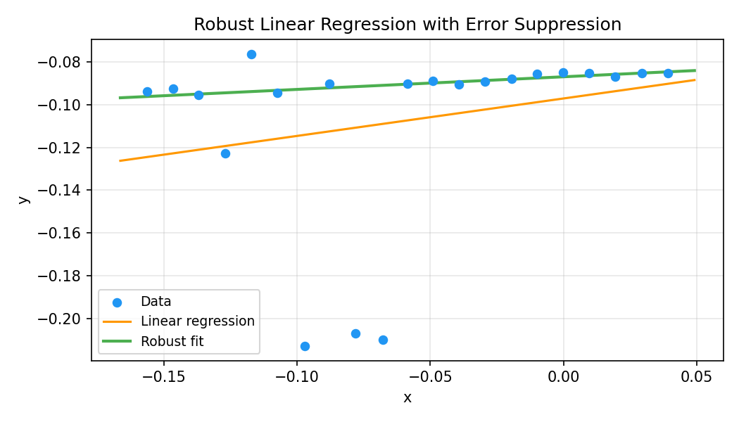
## Starship robust error suppression
Every residual above is wrapped in $\gamma \arctan(r / \gamma)$. This is the **Starship method** ([US Patent 12,346,118](https://patents.google.com/patent/US12346118)) -- a way to cap how much a single outlier can move the optimum without losing smooth differentiability. This section explains what it does and why.
### Setup
Given sensor readings stacked into a vector $L$, model parameters $M$ (poses, landmarks, etc.), and a prediction $\mu(M)$ of what the sensors should report given $M$, Bayesian inference with $L \mid M \sim \mathcal{N}(\mu(M), K_L)$ -- where $K_L$ is the sensor covariance matrix -- leads to minimising the sum
$$
S(M) = (L - \mu(M))^T K_L^{-1} (L - \mu(M)).
$$
**Whitening.** Diagonalising $K_L = R D R^T$ and substituting $L^D = R^T L$, $G(M) = R^T \mu(M)$ turns the quadratic form into a plain sum of squares in units of standard deviations:
$$
S(M) = \sum_i r_i^2, \qquad r_i = \frac{L_i^D - G_i(M)}{\sigma_i}.
$$
The solver minimises $S(M)$ (the Gauss-Newton / LM step), and every inner term $r_i$ is dimensionless -- a pure sigma count.
### The outlier problem
Each $r_i^2$ grows as the *square* of the measurement error. A single bad association at $10\sigma$ already contributes $100$ to the sum; at $30\sigma$ it contributes $900$. A handful of bad measurements drown out the signal from hundreds of good ones and pull the optimum off.
The usual robust-loss fixes -- L1 ($|r|$) and Huber (quadratic near zero, linear past a threshold) -- replace $r^2$ with something that grows slower than quadratically, which limits but does not cap each residual's contribution; a single very bad outlier can still pull the solution. Their derivatives are also awkward: L1 has a kink at $r = 0$ (undefined derivative there), Huber has a kink at the quadratic-to-linear transition (continuous but not smooth), and Gauss-Newton wants a smooth Jacobian. We want a loss that is both fully bounded and smooth everywhere.
### The cap
We look for a function $\alpha(x)$ that behaves like $x$ in the normal range but saturates for large inputs, so that $\alpha(x)^2$ contributes a bounded amount $\Delta S_{\max}$ to the sum instead of an unbounded $x^2$.
A clean choice is
$$
\alpha(x) = \gamma \arctan\frac{x}{\gamma}, \qquad \gamma = \frac{2 \sqrt{\Delta S_{\max}}}{\pi}.
$$
The $\gamma$ value follows from the saturation requirement: as $|x| \to \infty$, $\arctan(x/\gamma) \to \pm \pi/2$, so $\alpha(x)^2 \to (\gamma \pi / 2)^2$; setting that equal to $\Delta S_{\max}$ and solving gives the $\gamma$ above. Three further properties fall out:
- $\alpha(x) \approx x$ for $|x| \sim 1$ -- small residuals pass through unchanged.
- $\alpha'(0) = 1$, so near the optimum the loss is indistinguishable from plain $r^2$.
- $\alpha(x)^2 \to \Delta S_{\max}$ as $|x| \to \infty$ -- no single residual can push the sum by more than $\Delta S_{\max}$.

Left: $\alpha(x)$ (green) bends away from the identity $x$ (purple) once $|x|$ moves past a few sigmas. Right: the *squared* contribution -- the unbounded $x^2$ parabola vs the saturating $\alpha(x)^2$, capped at $\Delta S_{\max}$. The cap is also smooth; Gauss-Newton still sees a well-defined Jacobian everywhere.
### Using it
Replace each $r_i$ in the sum with $\alpha(r_i)$:
$$
\hat{S}(M) = \sum_i \alpha(r_i)^2 = \sum_i \left[ \gamma \arctan\frac{L_i^D - G_i(M)}{\gamma \sigma_i} \right]^2.
$$
In practice $\Delta S_{\max}$ in the range $[10, 25]$ (so $\gamma$ between roughly $2$ and $3$) suppresses genuine outliers hard without biasing inlier-dominated regions. Since residuals are already sigma-scaled, this corresponds roughly to saying "residuals past $3$ to $5\sigma$ stop mattering".
In arael this is exactly what you see in the demo constraint bodies:
```rust
let plain_r = (a * e.x + b - e.y) / sigma;
gamma * atan(plain_r / gamma)
```
The symbolic-differentiation pipeline handles `atan`'s derivative automatically; from the macro's point of view the residual is just another expression. No special-case code, no outlier bookkeeping.
### Initialisation matters
Gauss-Newton (and Levenberg-Marquardt) is a local method: each step linearises the cost around the current $M$ and moves in the direction that linearisation suggests. For any loss, you need a starting $M_0$ close enough to the optimum that the linearisation is informative.
Starship makes this requirement stricter. The gradient falls off as $\alpha'(r) = 1 / (1 + \pi^2 r^2 / (4 \Delta S_{\max}))$, so at the recommended $\Delta S_{\max} = 25$ a residual at $5\sigma$ still carries about 29% of its least-squares pull and a $10\sigma$ residual about 9% -- still usable. Once you get out to $20\sigma$ and beyond it drops under 3% and those residuals are effectively frozen. If $M_0$ puts many residuals that far out, the solver has nothing to work with and stalls. The usual remedy is **graduated optimisation**: start with a large $\Delta S_{\max}$ (loose cap, everything in the informative regime), solve, then shrink it across passes down to the target value. The SLAM demo does this via a `frine_isigma_scale` field stepped per pass.
### Graduated passes in this demo
1. **Pass 1** (scale=0.01): Features contribute almost nothing. GPS, odometry, tilt, and drift dominate and find roughly correct poses.
2. **Pass 2** (scale=0.1): Features start pulling. Outliers are already suppressed by the robust cap.
3. **Pass 3** (scale=1.0): Full feature weight. Fine-tunes the solution. Outliers are deep in the `atan` saturation region and contribute at most $\Delta S_{\max}$ each.
## Uncertainty estimation
After optimization, the demo estimates landmark position uncertainty
from the inverse of the Gauss-Newton Hessian. The Hessian
`H = 2 * J^T * J` is the information matrix (the factor of 2 comes
from our cost function `sum(r^2)` without the conventional 1/2
prefactor). The parameter covariance matrix is:
```
Cov = (J^T * J)^{-1} = 2 * H^{-1}
```
### Global vs relative uncertainty
The raw diagonal block of `Cov` for a landmark gives its **global**
position uncertainty, which includes the gauge uncertainty (GPS
offset, yaw) shared by all parameters. This gauge floor dominates
and makes all landmarks look equally uncertain -- not useful.
The demo instead computes uncertainty **relative to the closest
pose**, which cancels the shared gauge. Given the full covariance
with blocks `C_ll` (landmark), `C_pp` (pose position), and `C_lp`
(cross-covariance):
```
Cov_rel = C_ll - C_lp - C_pl + C_pp
```
The eigendecomposition of this 3x3 `Cov_rel` yields three
eigenvalues whose square roots are the semi-axis lengths of the
**1-sigma uncertainty ellipsoid** -- an ellipsoid describing the
uncertainty of the landmark's position relative to the nearby pose.
The three eigenvectors give the principal directions of uncertainty.
Printed as `sigma=(a, b, c)` in descending order:
```
LM 227: |d|=0.017m rel=0.30% dist=5.8m sigma=(0.417,0.059,0.006)m frines=26
LM 224: |d|=0.054m rel=0.21% dist=25.9m sigma=(1.876,0.319,0.020)m frines=23
```
- The **largest** axis is depth (radial distance from observing
cameras), the hardest direction to constrain from angular
measurements alone. It scales roughly with landmark distance.
- The **middle** axis reflects the angular baseline of observations.
- The **smallest** axis is well-constrained by many observations
from different poses.
- More observations (`frines`) and wider baselines produce smaller
ellipsoids.
The dense Hessian inverse is `O(n^3)` and practical for the demo
problem size (n=1080). For larger problems, sparse
selected-inversion or Schur complement methods would be needed.
## Compile-time pipeline
```
Constraint expression (user writes)
|
v
Symbolic interpretation (proc macro interprets body)
|
v
Symbolic differentiation (d/d(each param))
|
v
Euler angles substitution (sin/cos -> precomputed fields)
|
v
Common Subexpression Elimination (iterative, factor-aware)
|
v
Rust code generation (precedence-aware, minimal parens)
|
v
Compiled evaluate code (inlined in calc_cost / calc_grad_hessian)
```
## Key macro attributes
| Attribute | Purpose |
|-----------|---------|
| `#[arael::model]` | Generate Model trait impl, Sym companion, PARAM_COUNT |
| `#[arael(root)]` | Trigger constraint code generation on root struct (f64 default) |
| `#[arael(root, f32)]` | Root with f32 precision (blocks, solver, all f32) |
| `#[arael(constraint(block, ...))]` | Define constraint expression on a struct |
| `#[arael(ref = path)]` | Auto-resolve Ref fields from a collection |
| `SimpleEulerAngleParam<T>` | Euler angles with precomputed sin/cos and rotation matrix |
| `EulerAngleParam<T>` | Gimbal-lock-free euler angles (delta around reference rotation) |
| `#[arael(skip)]` | Skip field in serialization |
| `guard = expr` | Conditional constraint evaluation |
| `parent = name` | Name the parent variable in constraint body |
## Viewing generated code
Use `cargo expand` to inspect the code the macros produce:
```bash
cargo expand --example slam_demo 2>&1 | less
```
The generated `calc_cost` method traverses all constraint
collections, evaluating CSE-optimized compiled code. Here is a
simplified fragment from the tilt constraint on Pose (the actual
output has more constraints and CSE intermediates):
```rust
fn calc_cost(&mut self, params: &[f64]) -> f64 {
arael::model::Model::update64(self, params);
let __self_ref = unsafe { &*(self as *const Self) };
let mut __cost = 0.0 as f64;
// Tilt constraint loop (simplified):
for __item in self.poses.iter_mut() {
let pose = &*__item;
let path = &*__self_ref;
let __r_0 = (pose.ea.work().x - pose.info.tilt_roll)
* path.tilt_isigma;
let __r_1 = (pose.ea.work().y - pose.info.tilt_pitch)
* path.tilt_isigma;
__cost += __r_0 * __r_0 + __r_1 * __r_1;
}
// Odometry constraint loop (with CSE intermediates):
for __frine in self.pose_pairs.iter() {
let prev = &self.poses[__frine.prev];
let cur = &self.poses[__frine.cur];
let path = &*__self_ref;
// CSE: shared subexpressions extracted across all 6 residuals
let __x19 = cur.pos.work().x - prev.pos.work().x;
let __x20 = cur.pos.work().z - prev.pos.work().z;
let __x21 = cur.pos.work().y - prev.pos.work().y;
// Precomputed rotation matrix used directly:
let __x6 = __x19 * prev.ea.rotation_matrix[0].x
+ __x21 * prev.ea.rotation_matrix[1].x
- __x20 * prev.ea.sincos.0.y
- cur.info.delta_pos.x;
// ... more intermediates, residuals, cost accumulation
}
__cost
}
```
The `calc_grad_hessian_*` methods follow the same structure but also
compute symbolic derivatives (with CSE applied across both residuals
and their Jacobians) and accumulate them into `SelfBlock` /
`CrossBlock` hessian blocks via `add_residual()`.
## Full source
See [examples/slam_demo.rs](../examples/slam_demo.rs).