Crate ruviz

Expand description

§Ruviz - High-Performance Rust Plotting Library

A modern, high-performance 2D plotting library for Rust that combines matplotlib’s comprehensiveness with Makie’s performance-oriented design, while maintaining Rust’s safety and ergonomics.

§Features

Performance-Oriented: Built for release-mode plotting workloads with benchmarkable output paths
Zero Unsafe Public API: Memory safety without compromising performance
29 Plot Types (33 with the 3d feature): basic, distribution, continuous, composition, polar, vector and hierarchical families, plus subplot layout helpers
Publication Quality: PNG/SVG export with custom themes
Large Dataset Support: Streaming-friendly data structures and practical downsampling workflows
Cross Platform: Linux, macOS, Windows
Animation Tooling: Frame-based recording plus signal-aware plot data APIs

§Quick Start

Every plot is built the same way: Plot::new(), one series method, setters, then save. There is no second entry point to learn.

use ruviz::prelude::*;

// Line plot
let x: Vec<f64> = (0..100).map(|i| i as f64 * 0.1).collect();
let y: Vec<f64> = x.iter().map(|&v| v.sin()).collect();
Plot::new().line(&x, &y).title("Sine Wave").save("sine.png")?;

// Scatter plot
Plot::new().scatter(&x, &y).title("Points").marker(MarkerStyle::Circle).save("scatter.png")?;

// Bar chart
let cats = ["A", "B", "C", "D"];
let vals = [10.0, 25.0, 15.0, 30.0];
Plot::new().bar(&cats, &vals).title("Sales").save("bar.png")?;

save finishes the pending series for you, so .end_series() is only needed when you want the Plot value itself — for example to hand it to subplots.

§Typst Text Mode

Enable Typst-backed labels and titles by turning on the typst-math feature:

[dependencies]
ruviz = { version = "0.4.16", features = ["typst-math"] }

Then opt into Typst text rendering per plot with .typst(true):

use ruviz::prelude::*;

let x: Vec<f64> = (0..50).map(|i| i as f64 * 0.1).collect();
let y: Vec<f64> = x.iter().map(|&v| (-v).exp()).collect();

let mut plot = Plot::new()
    .line(&x, &y)
    .title("$f(x) = e^(-x)$")
    .xlabel("$x$")
    .ylabel("$f(x)$");

#[cfg(feature = "typst-math")]
{
    plot = plot.typst(true);
}

plot.save("typst_plot.png")?;

If typst-math is not enabled, .typst(true) is unavailable and the compiler reports:

error[E0599]: no method named `typst` found for struct `ruviz::core::Plot` in the current scope

If Typst is optional in your own crate, define a local feature and forward it to ruviz/typst-math:

[dependencies]
ruviz = { version = "0.4.16", default-features = false }

[features]
default = []
typst-math = ["ruviz/typst-math"]

Then guard the call with #[cfg(feature = "typst-math")] in your crate. Selecting the text engine directly follows the same rule: TextEngineMode::Typst is only available when typst-math is enabled.

§Animation APIs

Create smooth animations with record! closures today. Signal-backed plot data and labels can also be attached to a plot. Plain render() and save() sample temporal sources at 0.0, while render_at() lets you choose the sampling time before using the normal backend-selection path. Push-based reactive sources use their latest value when the plot snapshot is built.

§Basic Animation with record! Macro

use ruviz::prelude::*;
use ruviz::record;

// Frame-based animation
record!("wave.gif", 60, |t| {
    let phase = t.time * 2.0 * std::f64::consts::PI;
    let x: Vec<f64> = (0..100).map(|i| i as f64 * 0.1).collect();
    let y: Vec<f64> = x.iter().map(|&xi| (xi + phase).sin()).collect();
    Plot::new().line(&x, &y).title(format!("t = {:.2}s", t.time))
})?;

// Duration-based animation (2 seconds at 30fps)
record!("bounce.gif", 2 secs, |t| {
    let y = t.ease_over(easing::ease_out_bounce, 100.0, 0.0, 2.0);
    Plot::new().scatter(&[0.0], &[y]).title("Bouncing Ball")
})?;

// Custom framerate
record!("smooth.gif", 3 secs @ 60 fps, |t| {
    let x = t.lerp_over(0.0, 10.0, 3.0);
    Plot::new().line(&[0.0, x], &[0.0, x]).title("Growing Line")
})?;

§Signals Inside Animation Closures

Use Signal<T> to build time-varying values, then sample them inside record! closures for animated series data today:

use ruviz::prelude::*;
use ruviz::animation::signal;
use ruviz::record;

// Create signals that vary over time
let amplitude = signal::lerp(0.0, 2.0, 3.0);  // 0 to 2 over 3 seconds
let frequency = signal::ease(easing::ease_in_out_quad, 1.0, 5.0, 3.0);

// Compose signals
let x: Vec<f64> = (0..100).map(|i| i as f64 * 0.1).collect();
let y_signal = signal::of(move |t| {
    let amp = amplitude.at(t);
    let freq = frequency.at(t);
    (0..100).map(|i| {
        let x = i as f64 * 0.1;
        amp * (x * freq).sin()
    }).collect::<Vec<f64>>()
});

// Use a signal-backed title alongside the sampled series data
let title = signal::of(|t| format!("Wave Animation - t={:.2}s", t));

record!("wave.gif", 3 secs, |t| {
    let y = y_signal.at(t);
    Plot::new()
        .title(title.at(t))
        .line(&x, &y)
})?;

§Reactive Labels

Attach signal-backed titles and axis labels:

use ruviz::prelude::*;
use ruviz::animation::signal;

// Dynamic title showing current time
let title = signal::of(|t| format!("Simulation: {:.1}s", t));

// Dynamic axis label
let ylabel = signal::of(|t| {
    if t < 1.0 { "Accelerating".to_string() }
    else if t < 2.0 { "Constant Velocity".to_string() }
    else { "Decelerating".to_string() }
});

let x: Vec<f64> = (0..100).map(|i| i as f64 * 0.1).collect();
let y: Vec<f64> = x.iter().map(|&xi| xi.sin()).collect();

let plot = Plot::new()
    .title_signal(title)
    .xlabel("Time")
    .ylabel_signal(ylabel)
    .line(&x, &y);

§Signal Composition

Combine multiple signals for complex animations:

use ruviz::animation::signal;

// Basic signal constructors
let constant = signal::constant(42.0);           // Always returns 42
let time = signal::time();                       // Returns current time
let linear = signal::lerp(0.0, 100.0, 2.0);     // Linear interpolation
let eased = signal::ease(easing::ease_out_bounce, 100.0, 0.0, 2.0);

// Transform signals
let doubled = linear.map(|v| v * 2.0);

// Combine two signals
let combined = signal::zip(linear.clone(), eased, |a, b| a + b);

// Combine three signals
let rgb = signal::zip3(
    signal::lerp(0.0, 255.0, 1.0),
    signal::lerp(255.0, 0.0, 1.0),
    signal::constant(128.0),
    |r, g, b| (r as u8, g as u8, b as u8)
);

// Custom signal from closure
let sine_wave = signal::of(|t| (t * std::f64::consts::TAU).sin());

§Gallery

Click any image to view full size. Expand sections below to see code examples.

§Plot Types



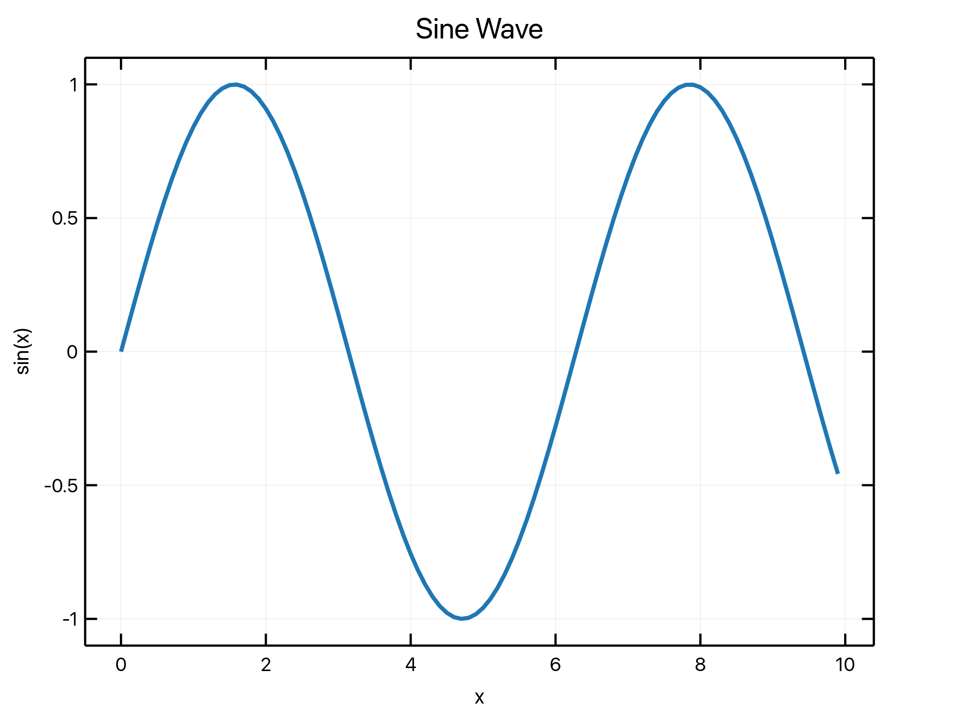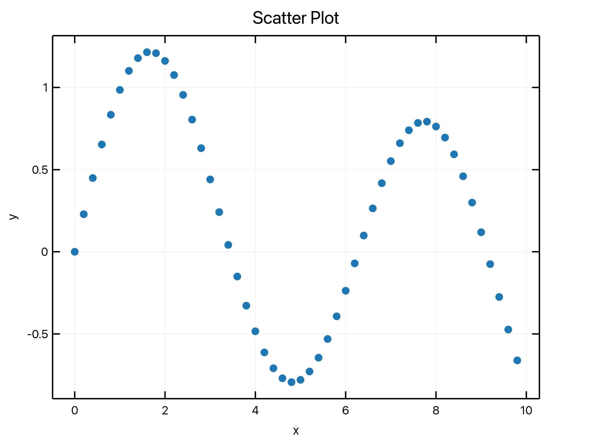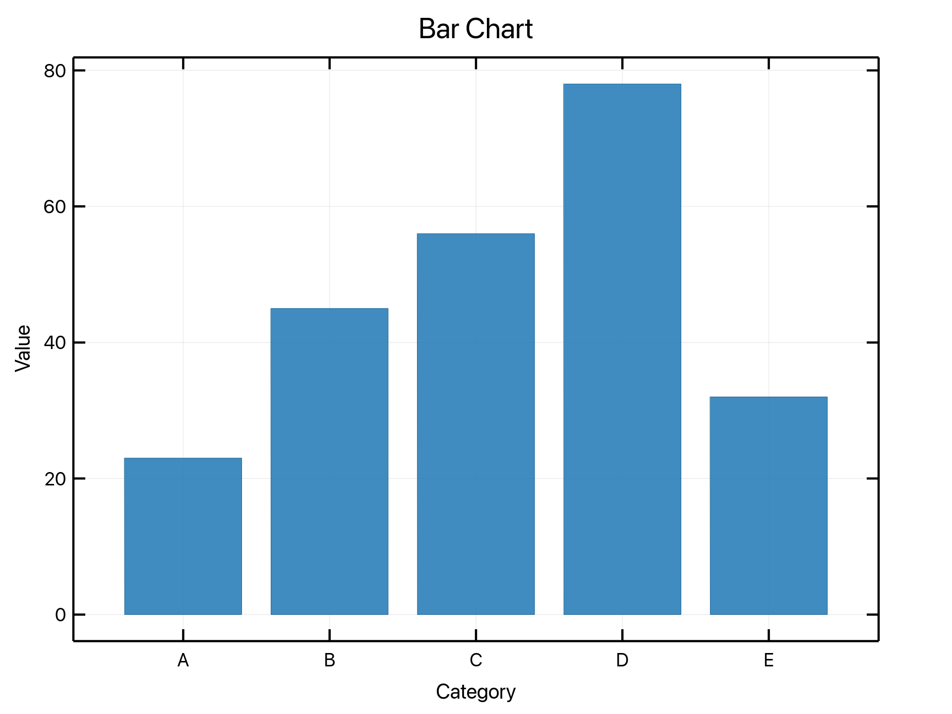Line Plot	Scatter Plot	Bar Chart

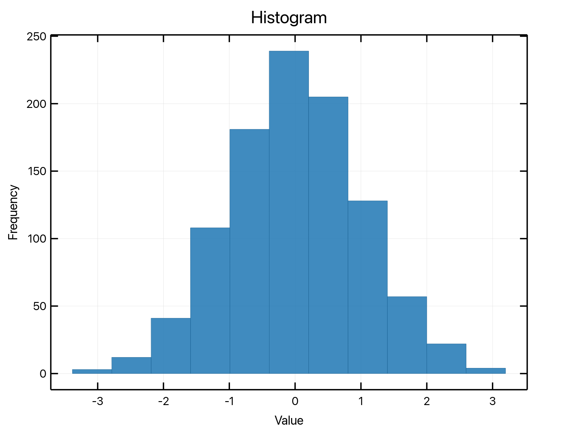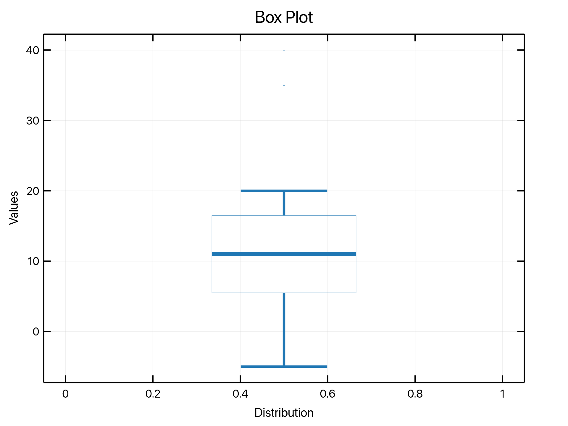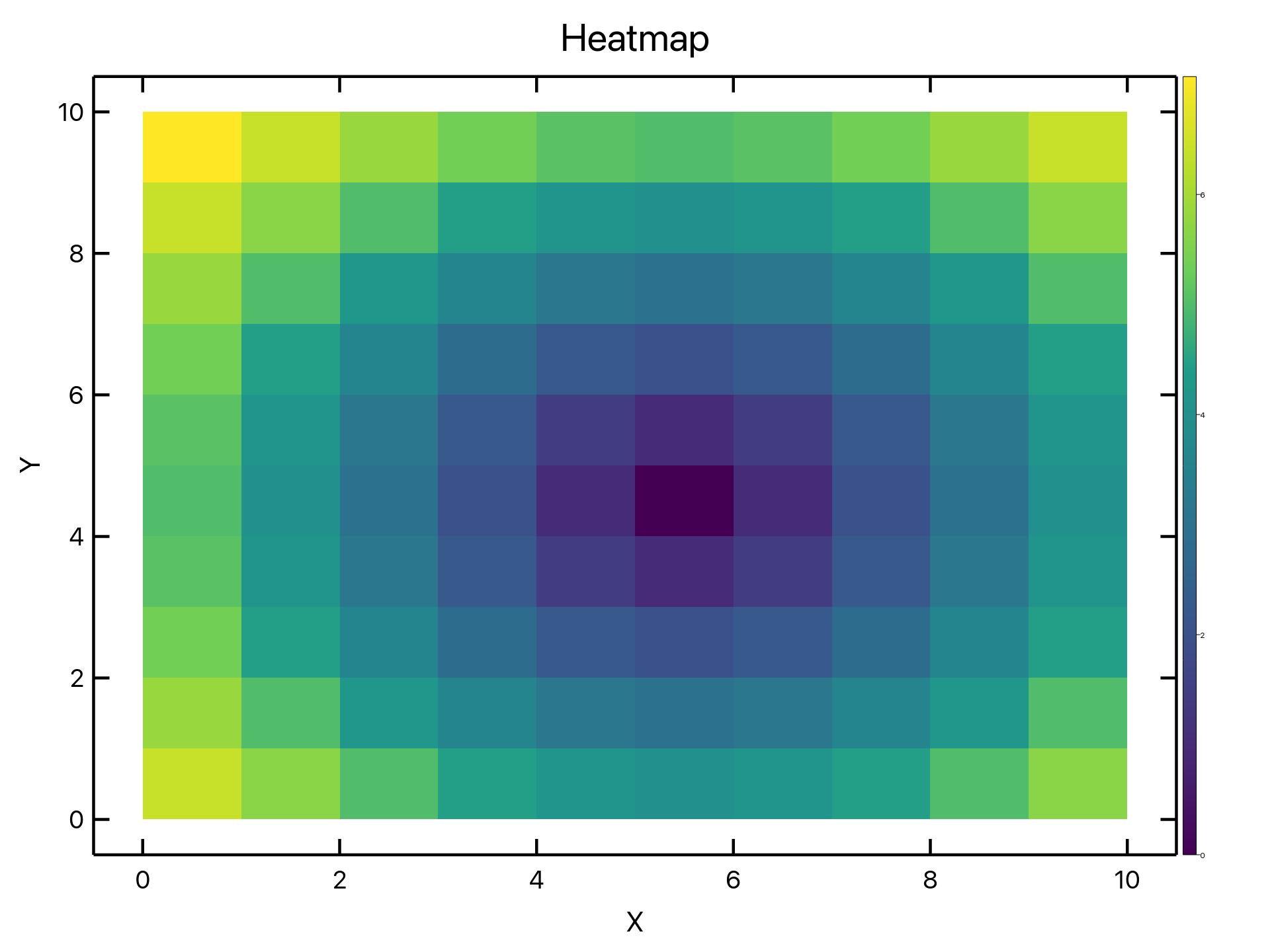Histogram	Box Plot	Heatmap

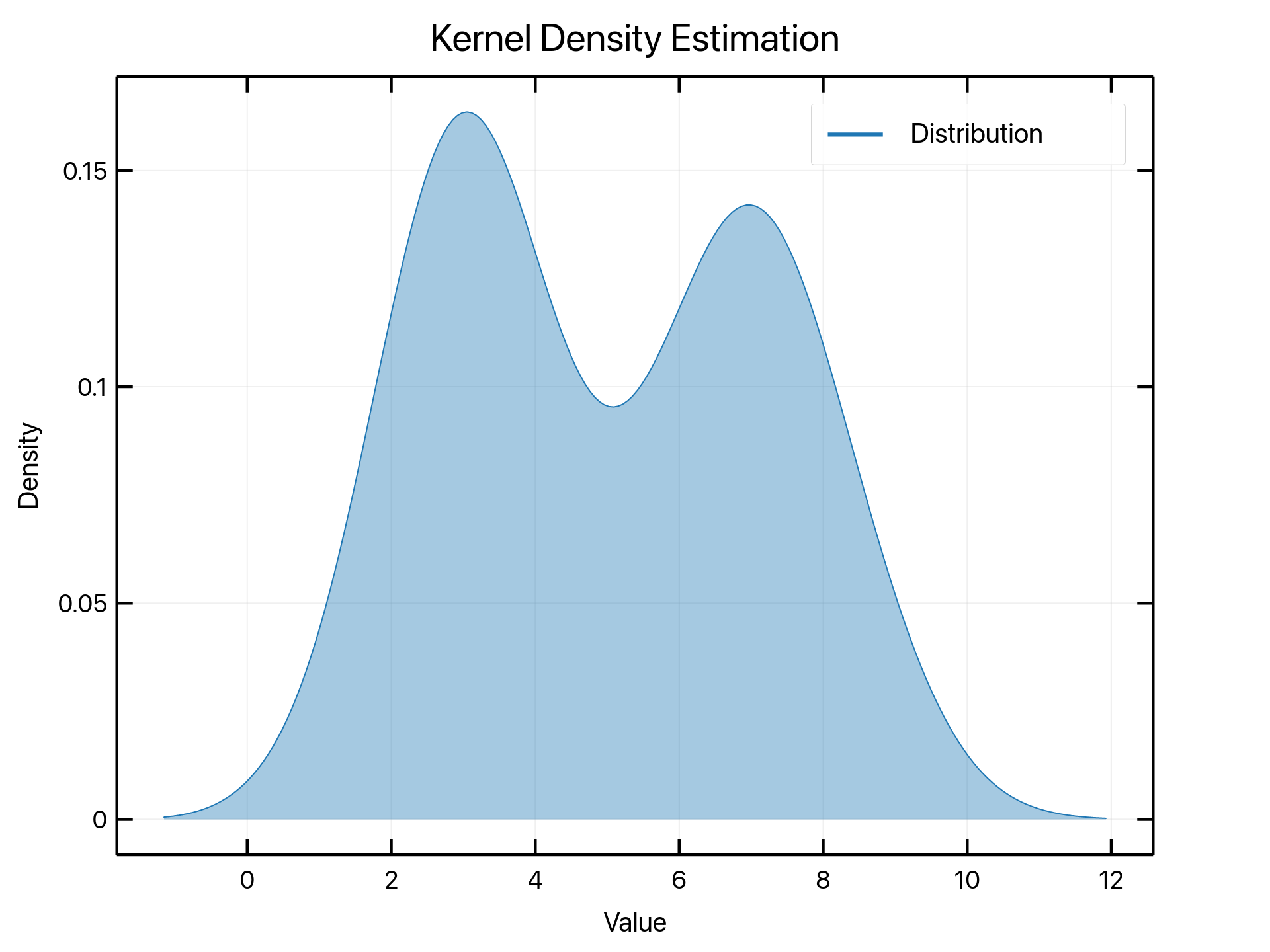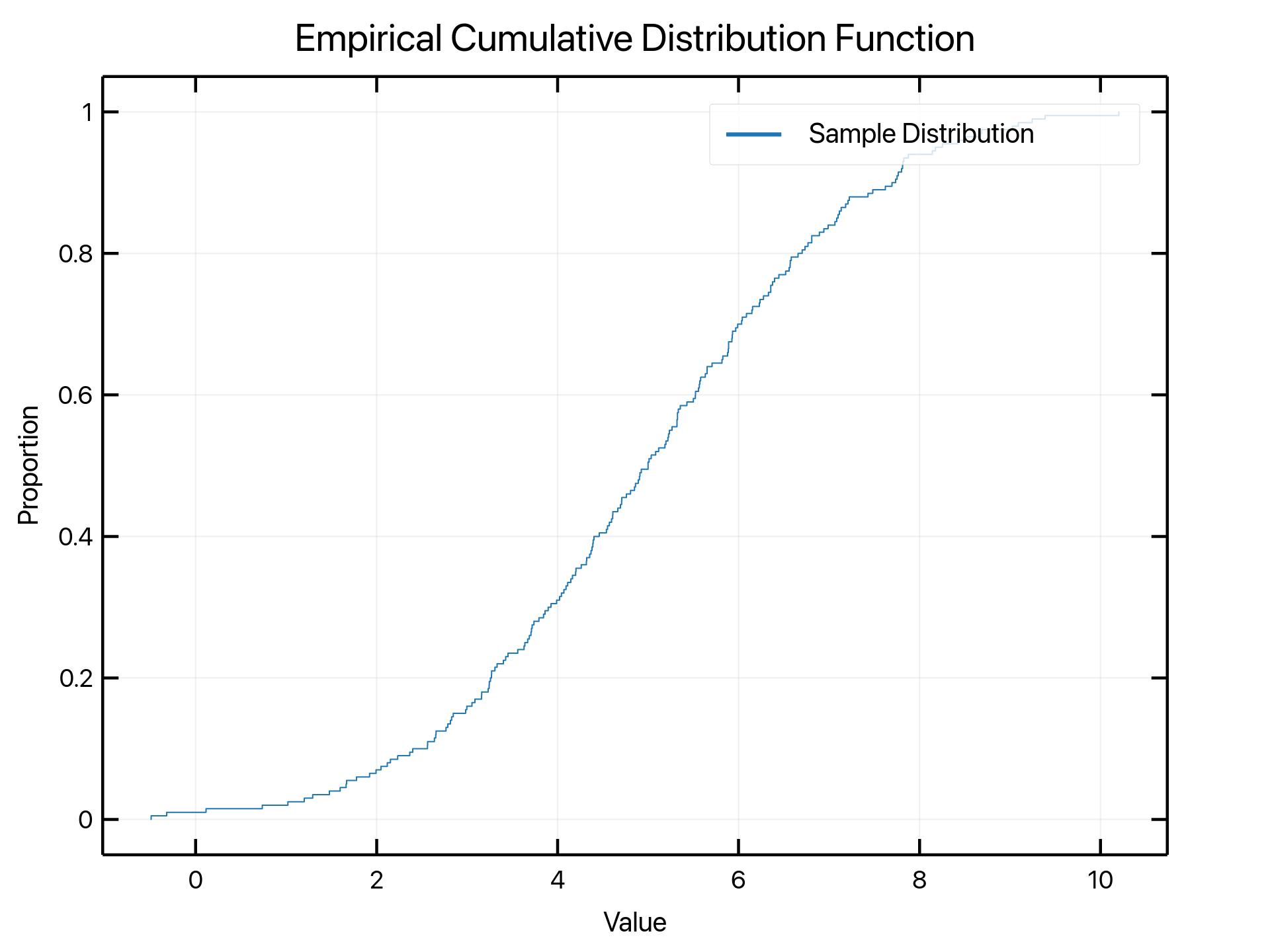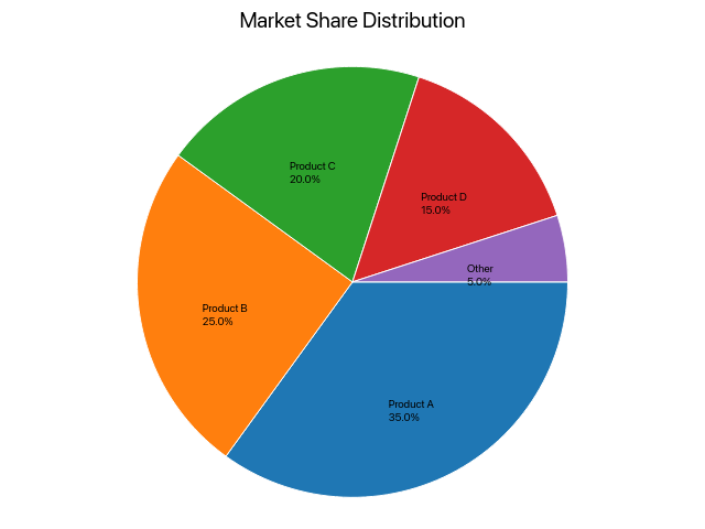KDE Plot	ECDF Plot	Pie Chart

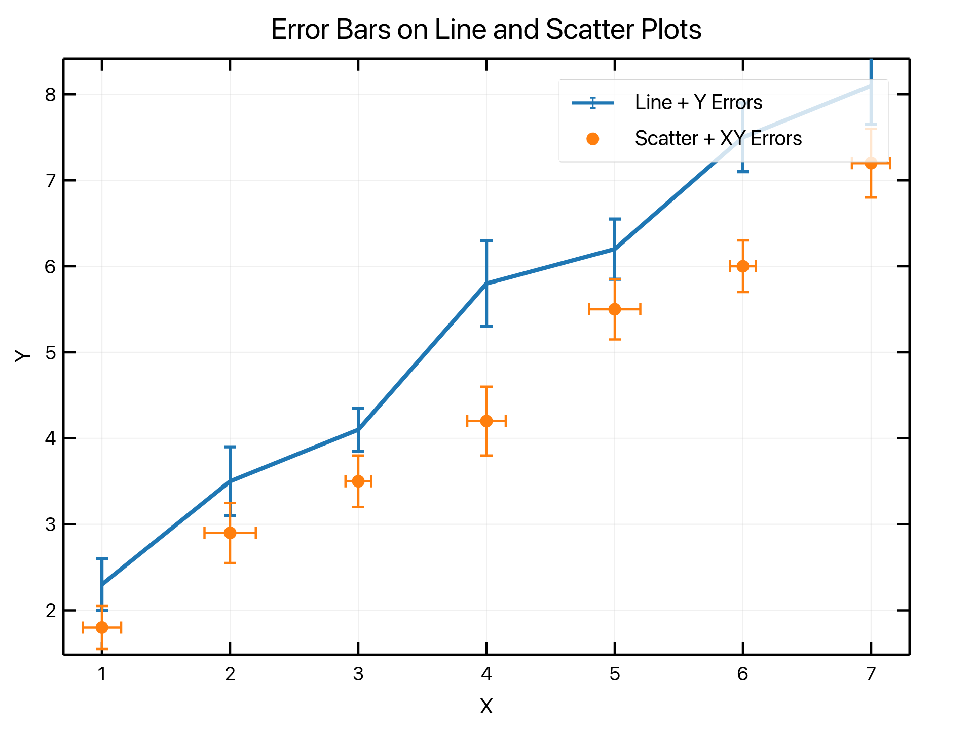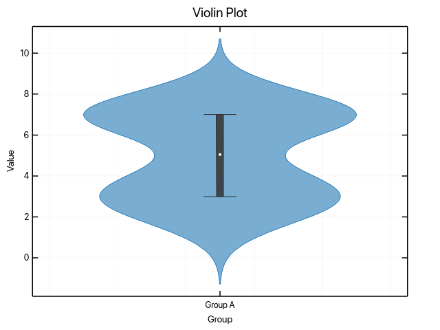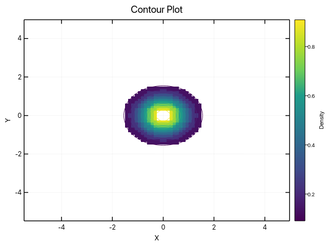Error Bar	Violin Plot	Contour Plot

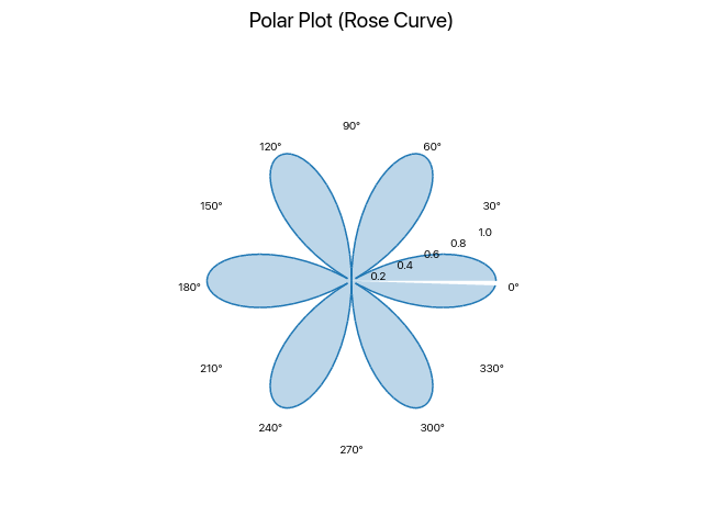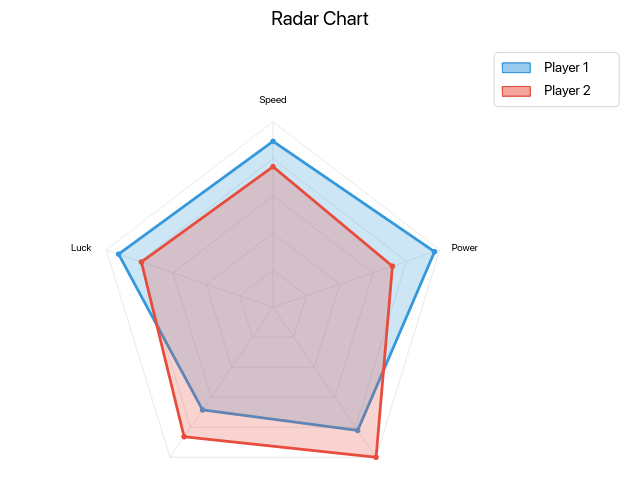Polar Plot	Radar Chart

§Additional Plot Types

The top-level Plot builder covers the most common scientific chart types:

Category	Plot Types
Basic	Line, Scatter, Bar
Distribution	Histogram, Box Plot, Violin, Boxen, KDE, ECDF, Rug, Strip, Swarm
Categorical (multi-series)	Grouped Bar, Stacked Bar
Continuous	Heatmap, Contour, Hexbin, Fill Between, Area, Stacked Area
Discrete	Step, Stem
Error	Error Bars
Composition	Pie, Donut
Polar	Polar Plot, Radar/Spider Chart
Vector	Quiver
Hierarchical	Dendrogram
3D (`3d` feature)	Scatter3D, Line3D, Surface3D, Wireframe3D

That is the complete list: 29 types from Plot, 4 more from Plot3D. src/plots/mod.rs::catalog_is_true reads the builder’s own source and fails if this table drifts from the API.

All of them except fill_between are series methods returning PlotBuilder<C>, so one chain works across every one: .<series>(..).label(..).color(..).legend_best().save(..). fill_between is an annotation rather than a series — it returns the plot itself, so it takes plot-level setters instead of series-level ones.

Joint plots and pair plots are figures rather than series: plots::composite::jointplot() and plots::composite::pairplot() return a SubplotFigure, like core::subplots does, so they are not counted above.

plots also exposes compute helpers (2D KDE, regression) that have no builder method and cannot be drawn — see the plots module docs. See the Plot Types Guide for details.

Plot Types Code Examples

Line Plot

use ruviz::prelude::*;

let x: Vec<f64> = (0..100).map(|i| i as f64 * 0.1).collect();
let y: Vec<f64> = x.iter().map(|&v| v.sin()).collect();

Plot::new()
    .title("Sine Wave")
    .xlabel("x")
    .ylabel("sin(x)")
    .line(&x, &y)
    .save("line_plot.png")?;

Scatter Plot

use ruviz::prelude::*;

let x: Vec<f64> = (0..50).map(|i| i as f64 * 0.2).collect();
let y: Vec<f64> = x.iter().enumerate()
    .map(|(i, &v)| v.sin() + (i as f64 * 0.1).sin() * 0.3)
    .collect();

Plot::new()
    .title("Scatter Plot")
    .xlabel("x")
    .ylabel("y")
    .scatter(&x, &y)
    .save("scatter_plot.png")?;

Bar Chart

use ruviz::prelude::*;

let categories = vec!["A", "B", "C", "D", "E"];
let values = vec![23.0, 45.0, 56.0, 78.0, 32.0];

Plot::new()
    .title("Bar Chart")
    .xlabel("Category")
    .ylabel("Value")
    .bar(&categories, &values)
    .save("bar_chart.png")?;

Histogram

use ruviz::prelude::*;

// Generate sample data
let data: Vec<f64> = (0..1000).map(|i| {
    let u1 = ((i * 7 + 13) % 1000) as f64 / 1000.0;
    let u2 = ((i * 11 + 17) % 1000) as f64 / 1000.0;
    (-2.0 * u1.max(0.001).ln()).sqrt() * (2.0 * std::f64::consts::PI * u2).cos()
}).collect();

Plot::new()
    .title("Histogram")
    .xlabel("Value")
    .ylabel("Frequency")
    .histogram(&data)
    .save("histogram.png")?;

Box Plot

use ruviz::prelude::*;

let data = vec![
    1.0, 2.0, 3.0, 4.0, 5.0, 6.0, 7.0, 8.0, 9.0, 10.0,
    11.0, 12.0, 13.0, 14.0, 15.0, 16.0, 17.0, 18.0, 19.0, 20.0,
    35.0, 40.0, -5.0,  // Outliers
];

Plot::new()
    .title("Box Plot")
    .xlabel("Distribution")
    .ylabel("Values")
    .boxplot(&data)
    .show_mean(true)
    .save("boxplot.png")?;

Heatmap

use ruviz::prelude::*;

// Create 2D data (distance from center, shifted positive for log scaling)
let data: Vec<Vec<f64>> = (0..10).map(|i| {
    (0..10).map(|j| {
        ((i as f64 - 5.0).powi(2) + (j as f64 - 5.0).powi(2)).sqrt() + 1.0
    }).collect()
}).collect();

Plot::new()
    .title("Log-Scaled Heatmap")
    .xlabel("X")
    .ylabel("Y")
    .heatmap(&data)
    .value_scale(AxisScale::Log)
    .colorbar_label("Distance")
    .save("heatmap.png")?;

§Styling Options



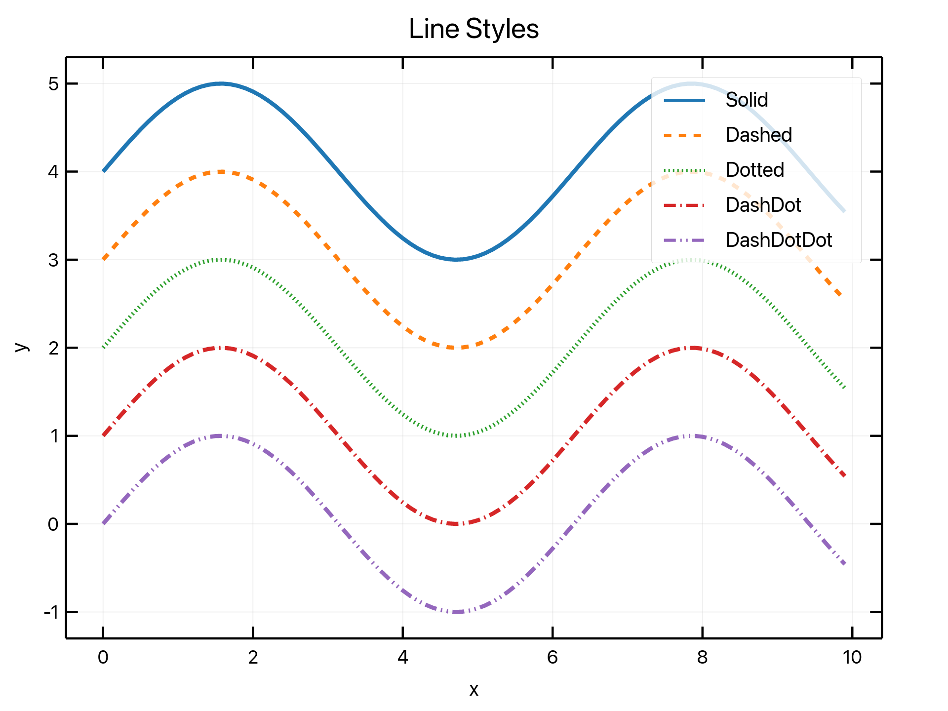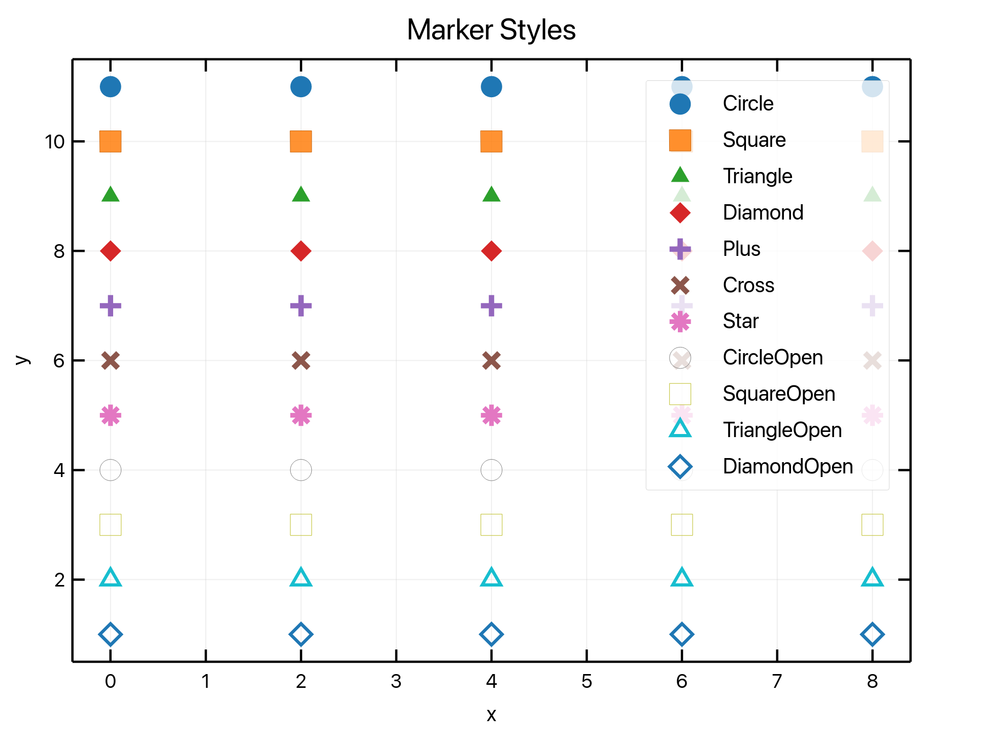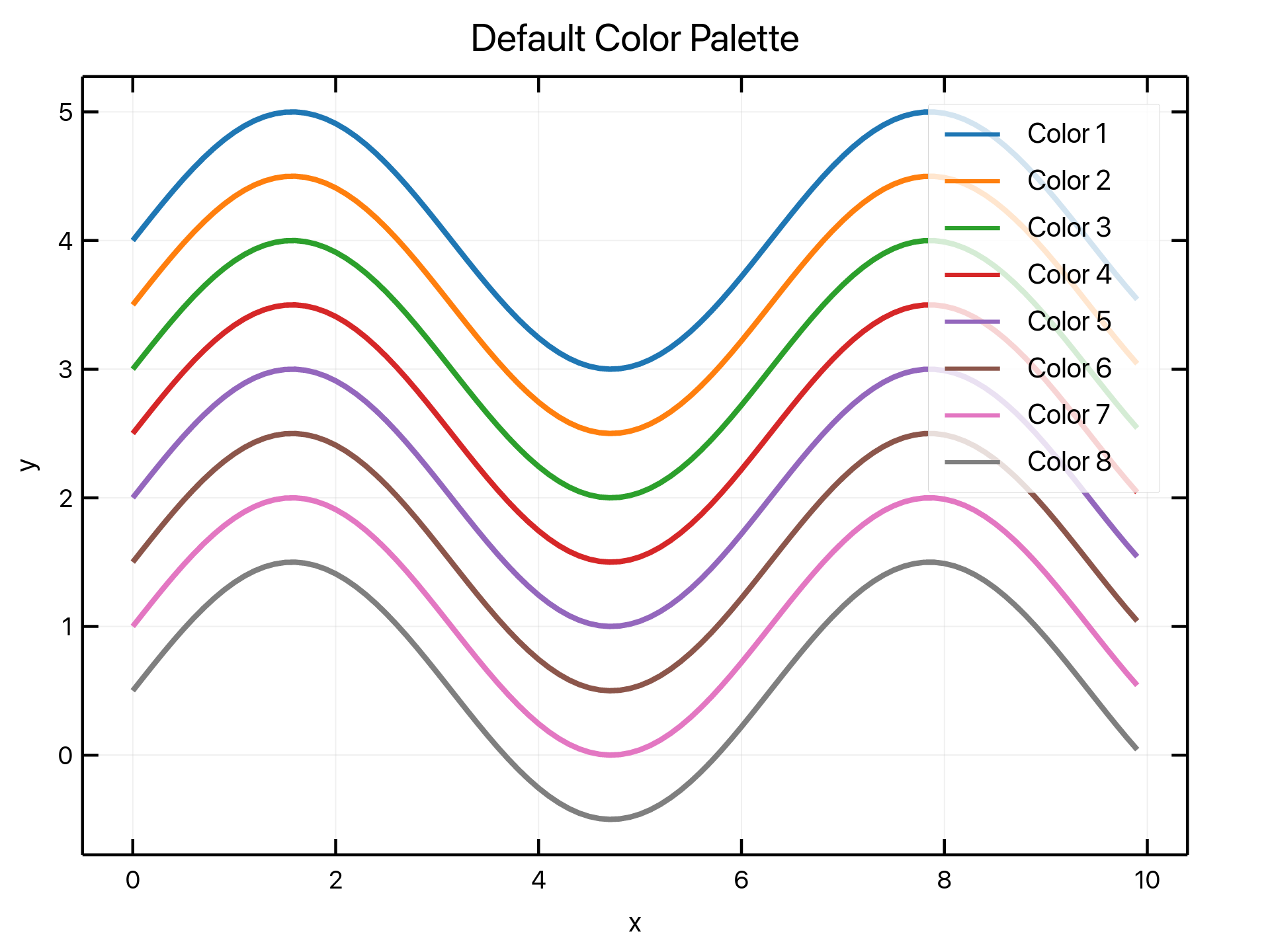Line Styles	Marker Styles	Color Palette

Styling Code Examples

Line Styles

use ruviz::prelude::*;

let x: Vec<f64> = (0..100).map(|i| i as f64 * 0.1).collect();

Plot::new()
    .title("Line Styles")
    .legend_position(LegendPosition::Best)
    .line(&x, &x.iter().map(|&v| v.sin() + 4.0).collect::<Vec<_>>())
    .label("Solid").line_style(LineStyle::Solid)
    .line(&x, &x.iter().map(|&v| v.sin() + 3.0).collect::<Vec<_>>())
    .label("Dashed").line_style(LineStyle::Dashed)
    .line(&x, &x.iter().map(|&v| v.sin() + 2.0).collect::<Vec<_>>())
    .label("Dotted").line_style(LineStyle::Dotted)
    .line(&x, &x.iter().map(|&v| v.sin() + 1.0).collect::<Vec<_>>())
    .label("DashDot").line_style(LineStyle::DashDot)
    .save("line_styles.png")?;

Marker Styles

use ruviz::prelude::*;

let x: Vec<f64> = (0..5).map(|j| j as f64 * 2.0).collect();

Plot::new()
    .title("Marker Styles")
    .legend_position(LegendPosition::Best)
    .scatter(&x, &vec![5.0; 5]).label("Circle").marker(MarkerStyle::Circle)
    .scatter(&x, &vec![4.0; 5]).label("Square").marker(MarkerStyle::Square)
    .scatter(&x, &vec![3.0; 5]).label("Triangle").marker(MarkerStyle::Triangle)
    .scatter(&x, &vec![2.0; 5]).label("Diamond").marker(MarkerStyle::Diamond)
    .scatter(&x, &vec![1.0; 5]).label("Star").marker(MarkerStyle::Star)
    .save("marker_styles.png")?;

Color Palette

use ruviz::prelude::*;

let palette = Color::default_palette();
let x: Vec<f64> = (0..100).map(|i| i as f64 * 0.1).collect();

Plot::new()
    .title("Default Color Palette")
    .legend_position(LegendPosition::Best)
    .line(&x, &x.iter().map(|&v| v.sin() + 3.0).collect::<Vec<_>>())
    .label("Color 1").color(palette[0])
    .line(&x, &x.iter().map(|&v| v.sin() + 2.0).collect::<Vec<_>>())
    .label("Color 2").color(palette[1])
    .line(&x, &x.iter().map(|&v| v.sin() + 1.0).collect::<Vec<_>>())
    .label("Color 3").color(palette[2])
    .line(&x, &x.iter().map(|&v| v.sin()).collect::<Vec<_>>())
    .label("Color 4").color(palette[3])
    .save("colors.png")?;

§Themes



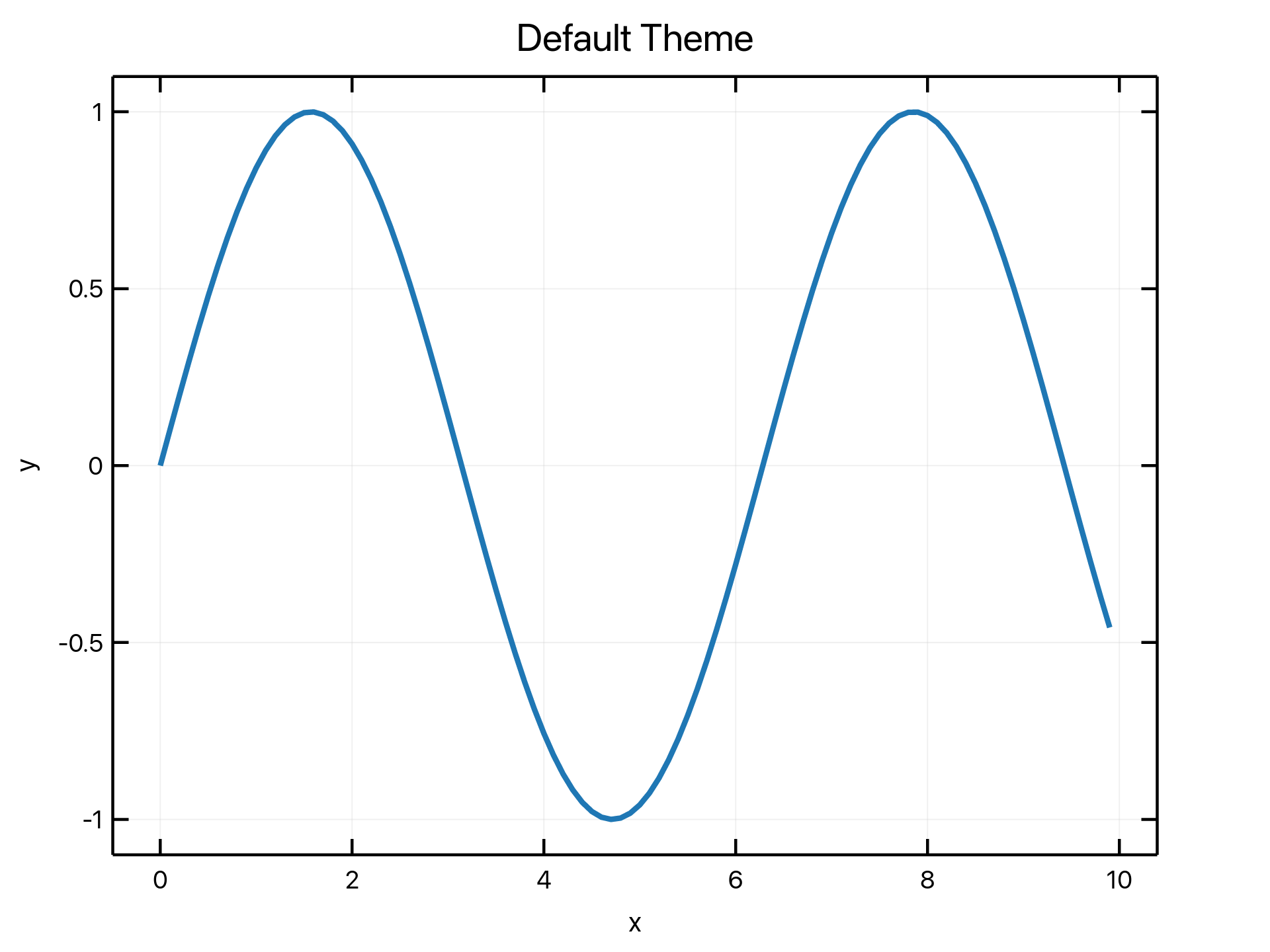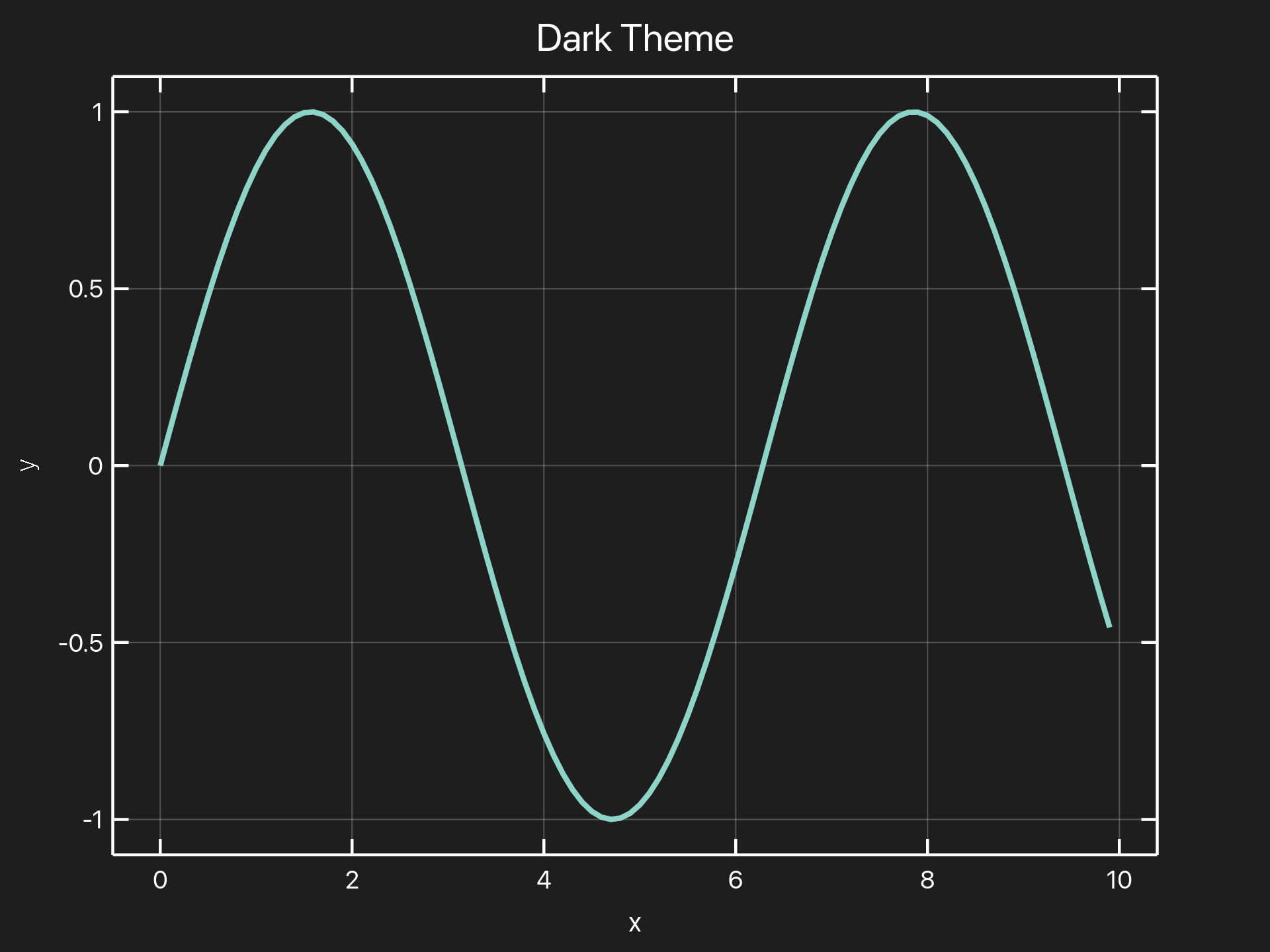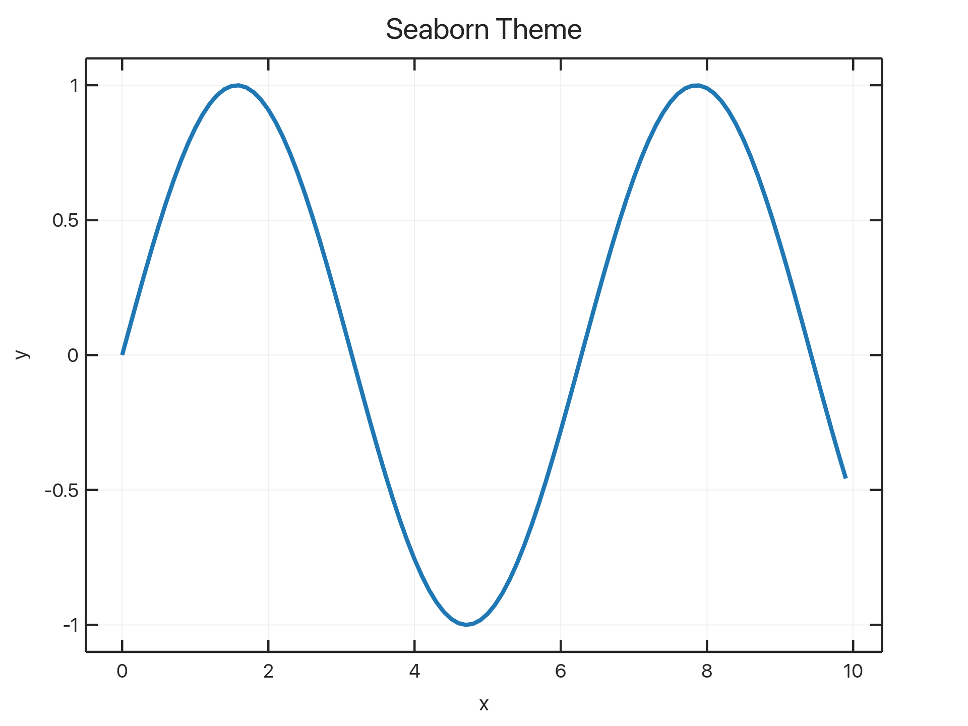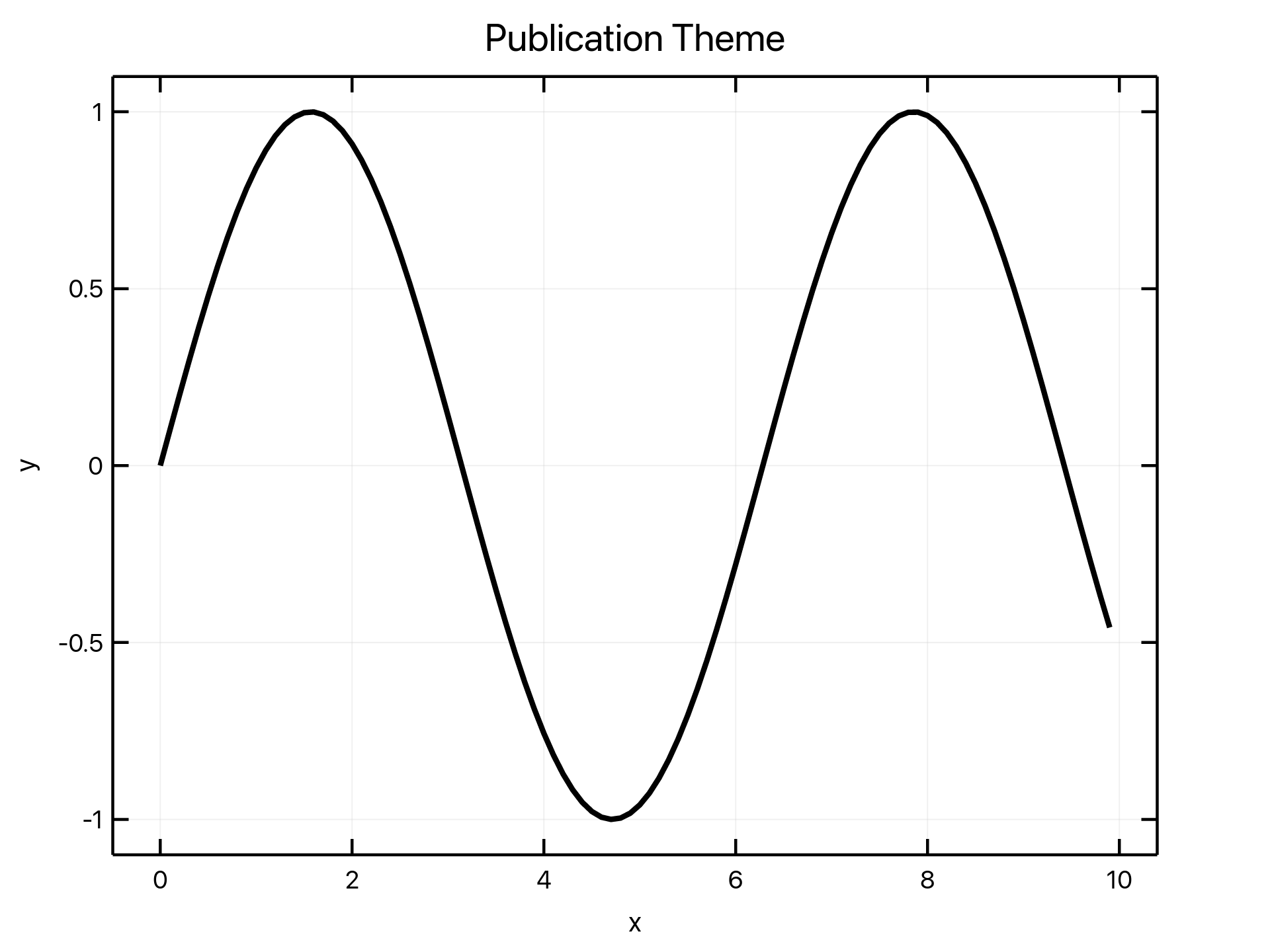Default	Dark	Seaborn	Publication

Themes Code Examples

Default Theme

use ruviz::prelude::*;

let x: Vec<f64> = (0..100).map(|i| i as f64 * 0.1).collect();
let y: Vec<f64> = x.iter().map(|&v| v.sin()).collect();

Plot::new()
    .title("Default Theme")
    .line(&x, &y)
    .save("theme_default.png")?;

Dark Theme

use ruviz::prelude::*;

let x: Vec<f64> = (0..100).map(|i| i as f64 * 0.1).collect();
let y: Vec<f64> = x.iter().map(|&v| v.sin()).collect();

Plot::new()
    .title("Dark Theme")
    .theme(Theme::dark())
    .line(&x, &y)
    .save("theme_dark.png")?;

Seaborn Theme

use ruviz::prelude::*;

let x: Vec<f64> = (0..100).map(|i| i as f64 * 0.1).collect();
let y: Vec<f64> = x.iter().map(|&v| v.sin()).collect();

Plot::new()
    .title("Seaborn Theme")
    .theme(Theme::seaborn())
    .line(&x, &y)
    .save("theme_seaborn.png")?;

Publication Theme

use ruviz::prelude::*;

let x: Vec<f64> = (0..100).map(|i| i as f64 * 0.1).collect();
let y: Vec<f64> = x.iter().map(|&v| v.sin()).collect();

Plot::new()
    .title("Publication Theme")
    .theme(Theme::publication())
    .line(&x, &y)
    .save("theme_publication.png")?;

§Layout



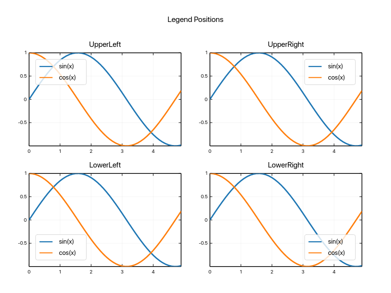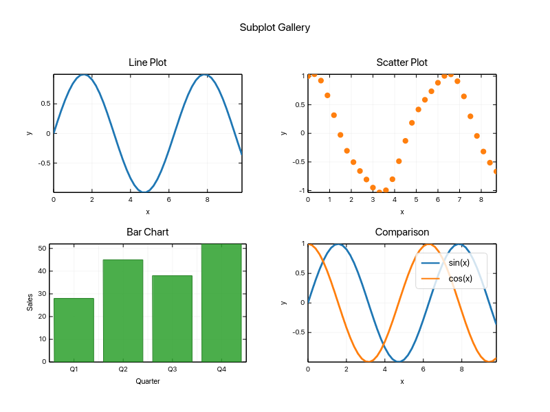Legend Positions	Subplots

Layout Code Examples

Legend Positions

use ruviz::prelude::*;

let x: Vec<f64> = (0..50).map(|i| i as f64 * 0.1).collect();
let y_sin: Vec<f64> = x.iter().map(|&v| v.sin()).collect();
let y_cos: Vec<f64> = x.iter().map(|&v| v.cos()).collect();

// Create plots with different legend positions
let plot_ul = Plot::new()
    .title("UpperLeft")
    .legend_position(LegendPosition::UpperLeft)
    .line(&x, &y_sin).label("sin(x)")
    .line(&x, &y_cos).label("cos(x)")
    .end_series();

let plot_ur = Plot::new()
    .title("UpperRight")
    .legend_position(LegendPosition::UpperRight)
    .line(&x, &y_sin).label("sin(x)")
    .line(&x, &y_cos).label("cos(x)")
    .end_series();

let plot_ll = Plot::new()
    .title("LowerLeft")
    .legend_position(LegendPosition::LowerLeft)
    .line(&x, &y_sin).label("sin(x)")
    .line(&x, &y_cos).label("cos(x)")
    .end_series();

let plot_lr = Plot::new()
    .title("LowerRight")
    .legend_position(LegendPosition::LowerRight)
    .line(&x, &y_sin).label("sin(x)")
    .line(&x, &y_cos).label("cos(x)")
    .end_series();

// Combine in 2x2 subplots
subplots(2, 2, 800, 600)?
    .suptitle("Legend Positions")
    .subplot_at(0, plot_ul)?
    .subplot_at(1, plot_ur)?
    .subplot_at(2, plot_ll)?
    .subplot_at(3, plot_lr)?
    .save("legend_positions.png")?;

Subplots

use ruviz::prelude::*;

let x: Vec<f64> = (0..50).map(|i| i as f64 * 0.2).collect();

let plot_line = Plot::new()
    .title("Line Plot")
    .line(&x, &x.iter().map(|&v| v.sin()).collect::<Vec<_>>())
    .end_series();

let plot_scatter = Plot::new()
    .title("Scatter Plot")
    .scatter(&x, &x.iter().map(|&v| v.cos()).collect::<Vec<_>>())
    .end_series();

let plot_bar = Plot::new()
    .title("Bar Chart")
    .bar(&["Q1", "Q2", "Q3", "Q4"], &[28.0, 45.0, 38.0, 52.0])
    .end_series();

let plot_multi = Plot::new()
    .title("Comparison")
    .legend_position(LegendPosition::UpperRight)
    .line(&x, &x.iter().map(|&v| v.sin()).collect::<Vec<_>>()).label("sin")
    .line(&x, &x.iter().map(|&v| v.cos()).collect::<Vec<_>>()).label("cos")
    .end_series();

subplots(2, 2, 800, 600)?
    .suptitle("Subplot Gallery")
    .subplot_at(0, plot_line)?
    .subplot_at(1, plot_scatter)?
    .subplot_at(2, plot_bar)?
    .subplot_at(3, plot_multi)?
    .save("subplots.png")?;

§Internationalization



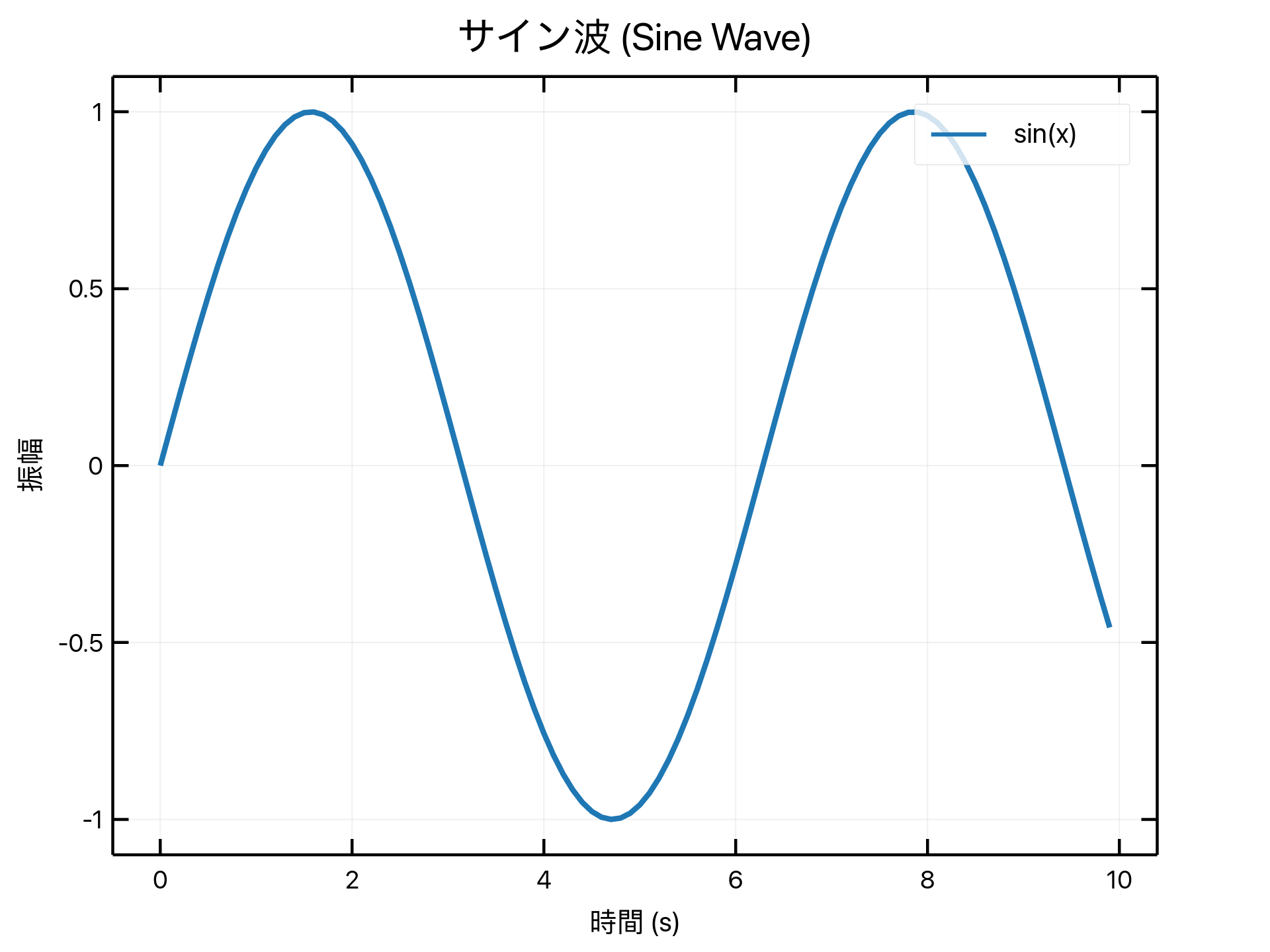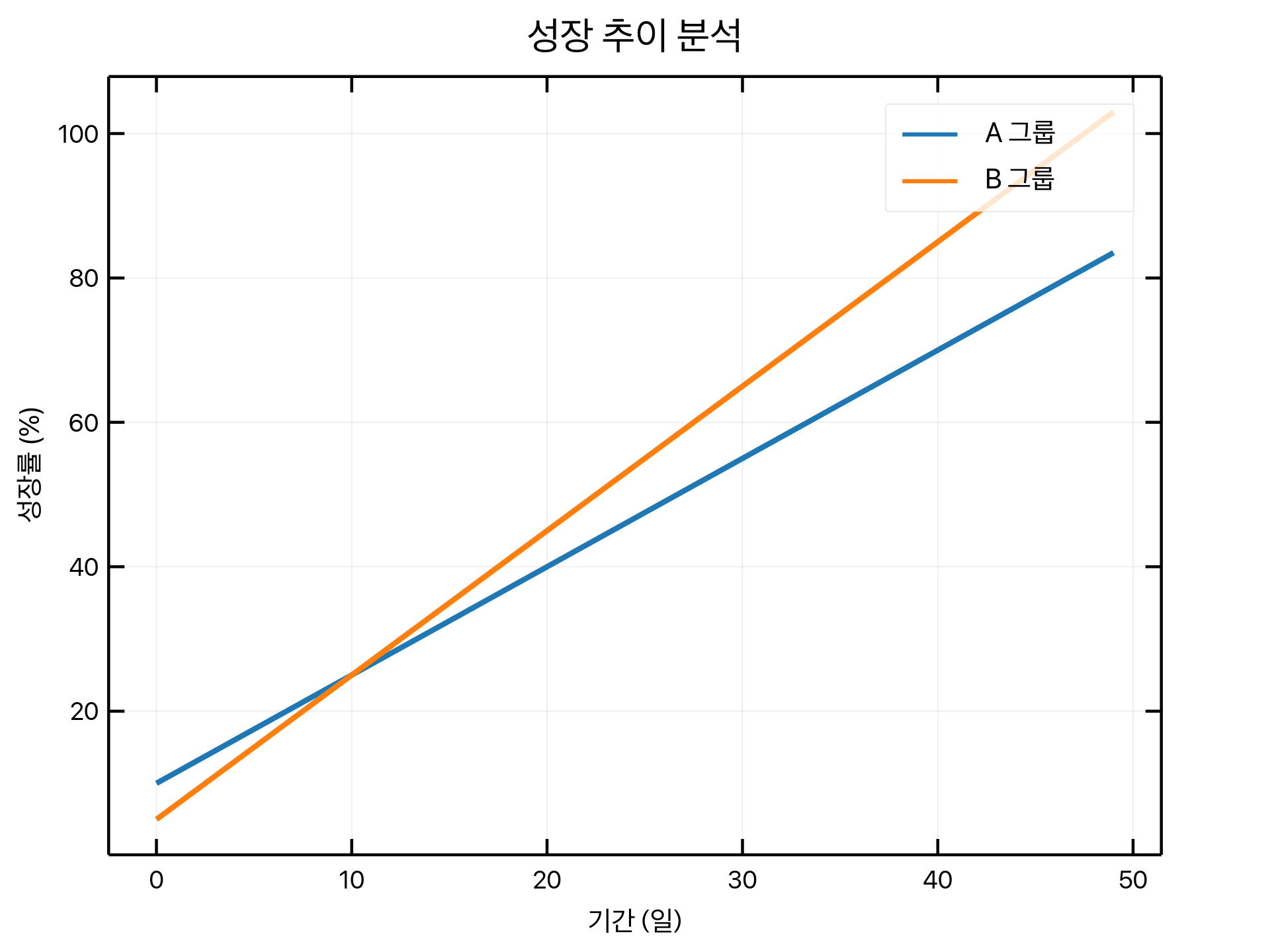日本語 (Japanese)	中文 (Chinese)	한국어 (Korean)

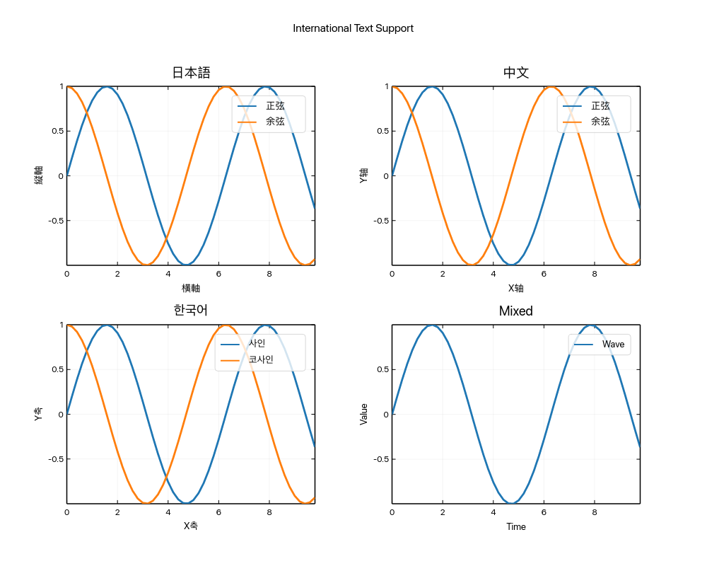Multi-language Comparison

Internationalization Code Examples

Japanese Labels

use ruviz::prelude::*;

let x: Vec<f64> = (0..100).map(|i| i as f64 * 0.1).collect();
let y: Vec<f64> = x.iter().map(|&v| v.sin()).collect();

Plot::new()
    .title("サイン波 (Sine Wave)")
    .xlabel("時間 (s)")
    .ylabel("振幅")
    .line(&x, &y)
    .label("sin(x)")
    .legend_best()
    .save("japanese_plot.png")?;

Chinese Labels

use ruviz::prelude::*;

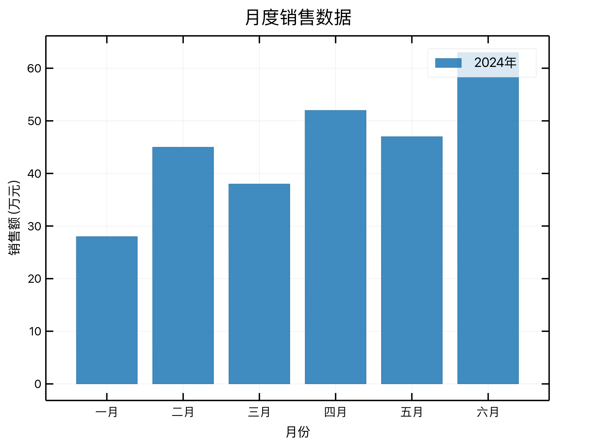
let categories = vec!["一月", "二月", "三月", "四月", "五月", "六月"];
let values = vec![28.0, 45.0, 38.0, 52.0, 47.0, 63.0];

Plot::new()
    .title("月度销售数据")
    .xlabel("月份")
    .ylabel("销售额 (万元)")
    .bar(&categories, &values)
    .save("chinese_plot.png")?;

§Animation

Smooth animations with the record! macro (requires animation feature):



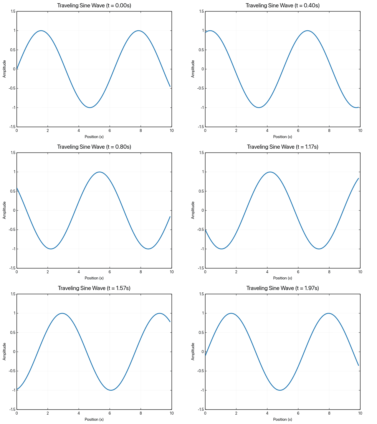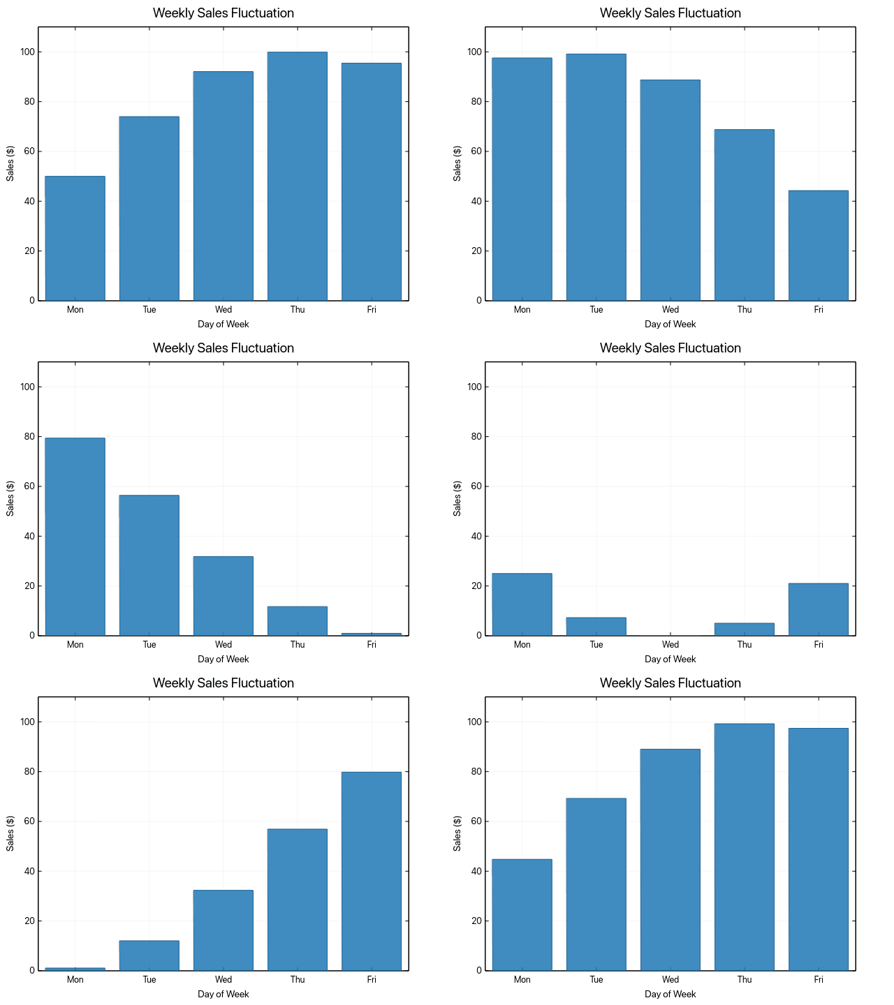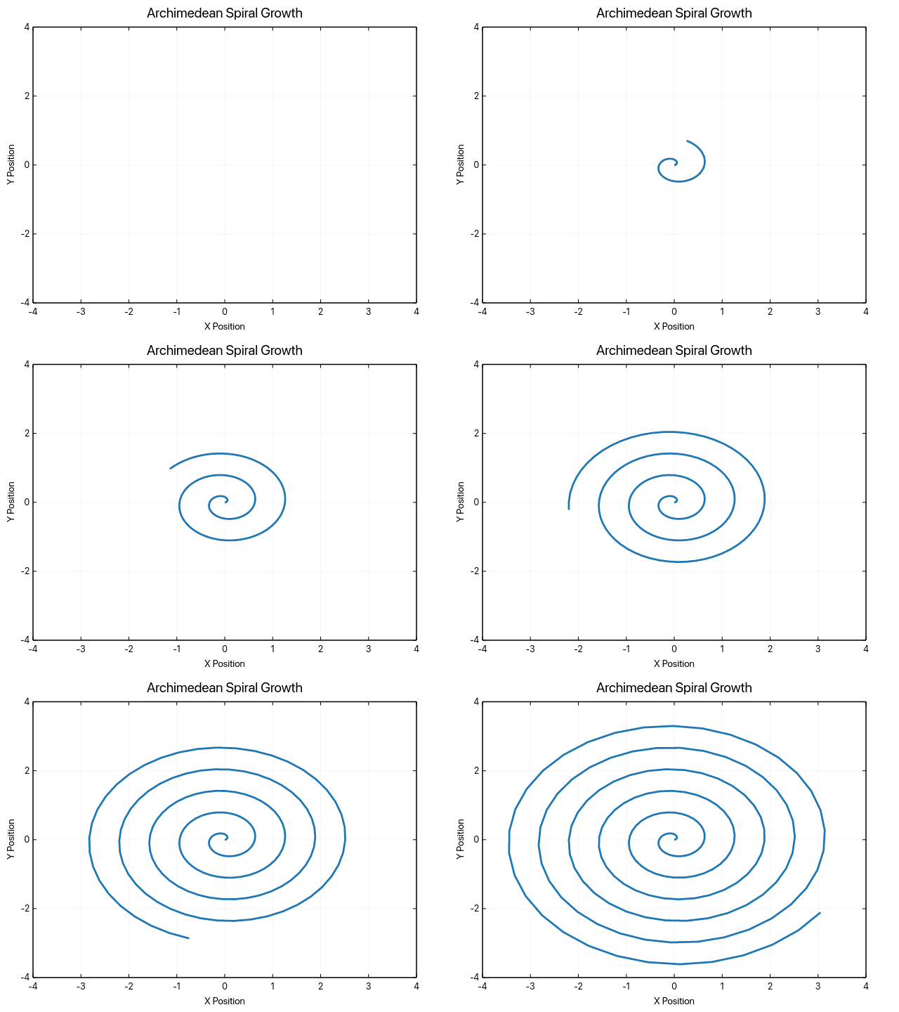Traveling Wave	Animated Bars	Spiral Growth

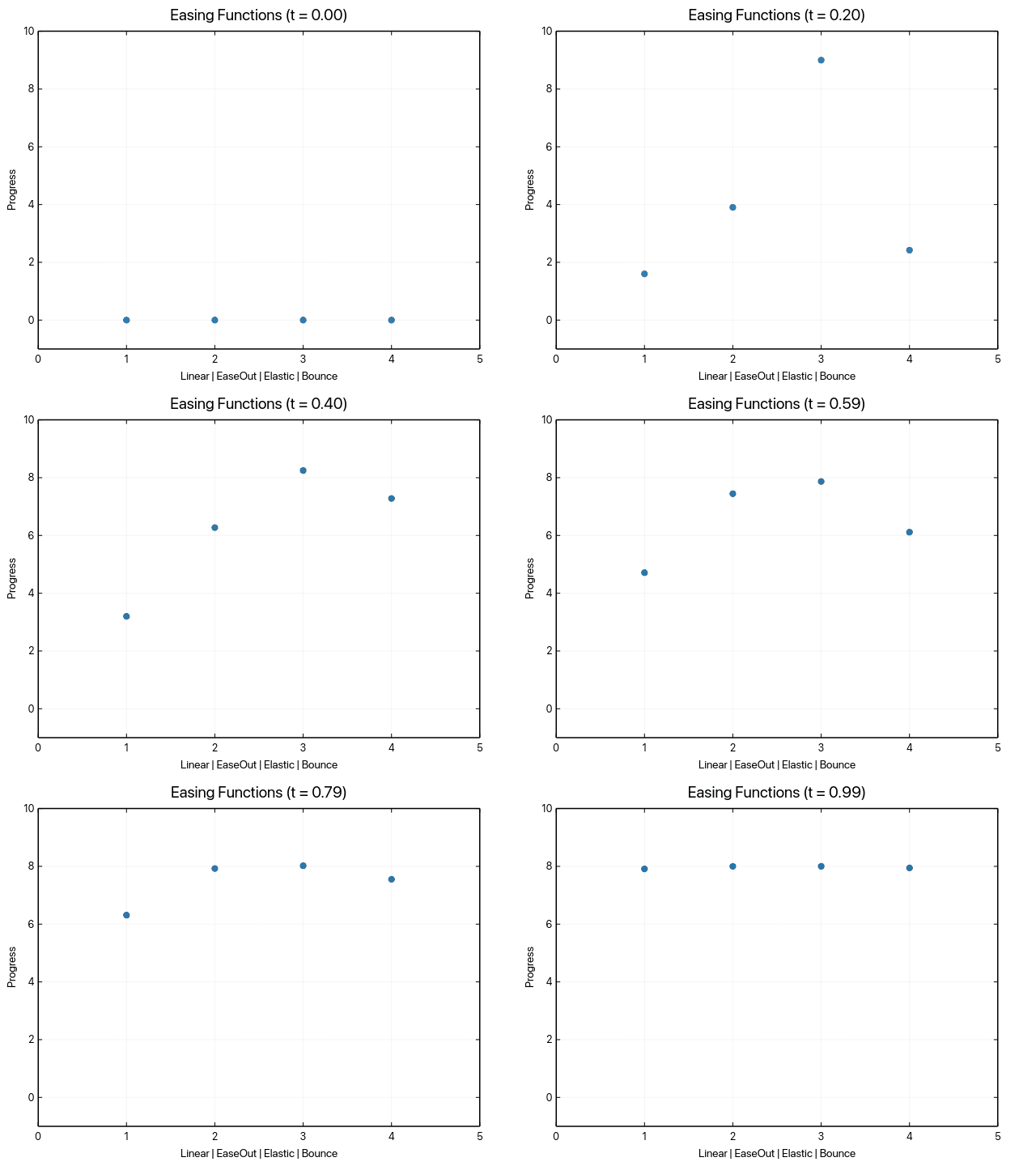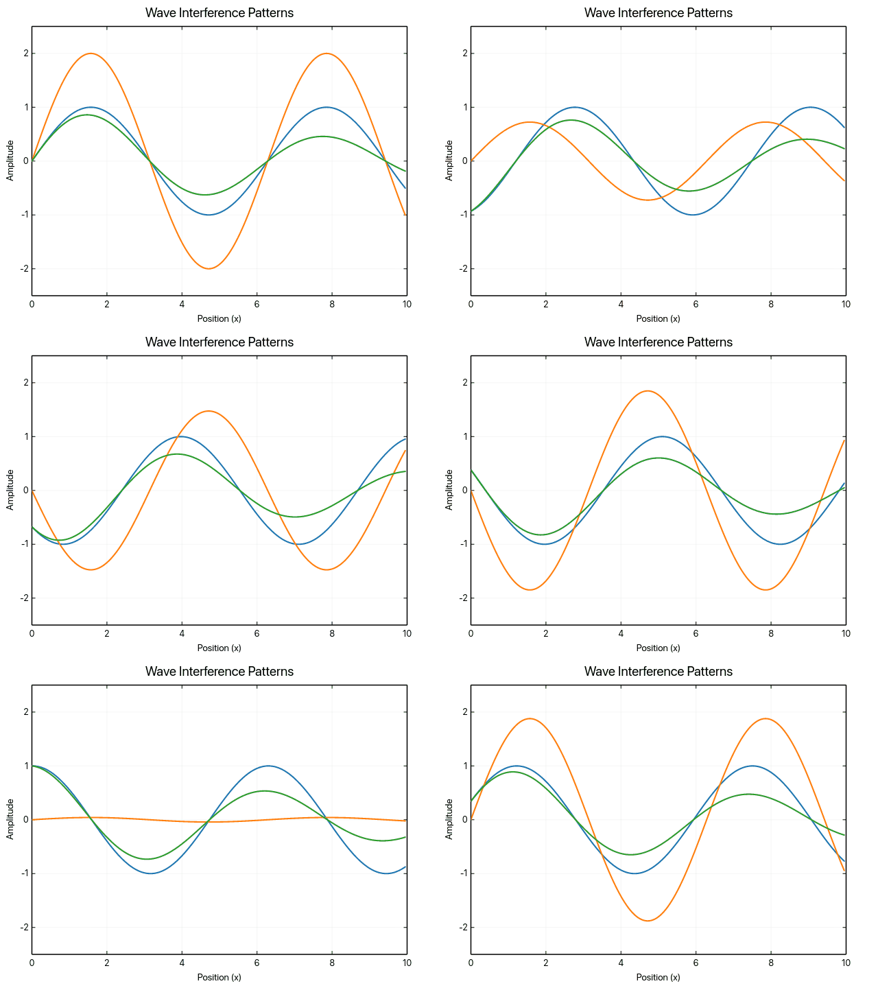Easing Functions	Wave Interference

See Animation Gallery for more examples.

§Common Tasks

Each of these is the same chain from Quick Start with one extra setter.

§Axis Labels

use ruviz::prelude::*;

let x = vec![0.0, 1.0, 2.0, 3.0, 4.0];
let y = vec![0.0, 1.0, 4.0, 9.0, 16.0];

Plot::new()
    .line(&x, &y)
    .title("Quadratic Function")
    .xlabel("x")
    .ylabel("y = x^2")
    .save("plot.png")?;

§With Legend (matplotlib-style)

Label each series, then enable the legend with legend_best() (the equivalent of plt.legend()) or legend_position(..) to place it yourself.

use ruviz::prelude::*;

let x: Vec<f64> = (0..100).map(|i| i as f64 * 0.1).collect();
let sin_y: Vec<f64> = x.iter().map(|&v| v.sin()).collect();
let cos_y: Vec<f64> = x.iter().map(|&v| v.cos()).collect();

Plot::new()
    .title("Trigonometric Functions")
    .line(&x, &sin_y).label("sin(x)")
    .line(&x, &cos_y).label("cos(x)")
    .legend_best()
    .save("trig.png")?;

§Figure Size and DPI

use ruviz::prelude::*;

let x: Vec<f64> = (0..100).map(|i| i as f64 * 0.1).collect();
let y: Vec<f64> = x.iter().map(|&v| v.sin()).collect();

Plot::new()
    .size(8.0, 6.0)  // 8×6 inches
    .dpi(300)        // 300 DPI = 2400×1800 pixels
    .line(&x, &y)
    .save("high_res.png")?;

§Named Colors

use ruviz::prelude::*;

let x: Vec<f64> = (0..50).map(|i| i as f64 * 0.2).collect();
let y: Vec<f64> = x.iter().map(|&v| v.sin()).collect();

// Use named colors (no unwrap needed!)
let color = Color::named("coral").unwrap_or(Color::RED);

Plot::new()
    .line(&x, &y).color(color)
    .save("colored.png")?;

Modules§

animationanimation and non-WebAssembly: Animation export system for ruviz
axes: Axis management and scaling
core: Core plotting functionality and main API
data: Data handling and trait definitions
export: Export functionality
layout: Layout and positioning
plots: Plot type implementations
prelude: Convenience re-exports for common usage
render: Rendering backend and styling
simpleNon-WebAssembly: Deprecated one-call plotting shortcuts.
stats: Statistical computations for advanced plot types
style: Unified style module for consistent theming and styling across all plot types
text: Text rendering and layout

Macros§

recordanimation and non-WebAssembly: Unified macro for animation recording.

Functions§

barDeprecated: Create a bar plot with the given categories and values.
lineDeprecated: Create a line plot with the given data.
line3d3d: Create a 3D line plot from x, y, and z coordinates.
scatterDeprecated: Create a scatter plot with the given data.
scatter3d3d: Create a 3D scatter plot from x, y, and z coordinates.
surface3d: Create a regular-grid surface where z.shape() == (y.len(), x.len()).
wireframe3d: Create a regular-grid wireframe where z.shape() == (y.len(), x.len()).

Crate ruviz

Crate ruviz Copy item path

§Ruviz - High-Performance Rust Plotting Library

§Features

§Quick Start

§Typst Text Mode

§Animation APIs

§Basic Animation with record! Macro

§Signals Inside Animation Closures

§Reactive Labels

§Signal Composition

§Gallery

§Plot Types

§Additional Plot Types

§Styling Options

§Themes

§Layout

§Internationalization

§Animation

§Common Tasks

§Axis Labels

§With Legend (matplotlib-style)

§Figure Size and DPI

§Named Colors

Modules§

Macros§

Functions§

Crate ruviz