Crate geopotential 

geopotential

Earth’s gravity field from spherical-harmonic coefficients. Read a model from an ICGEM .gfc file, from static models such as GOCO06s to every monthly GRACE field. Then evaluate the potential, the gravity vector or the gravity-gradient tensor at any point, or draw maps of the geoid, gravity anomalies or water height. Pure Rust, no required dependencies.

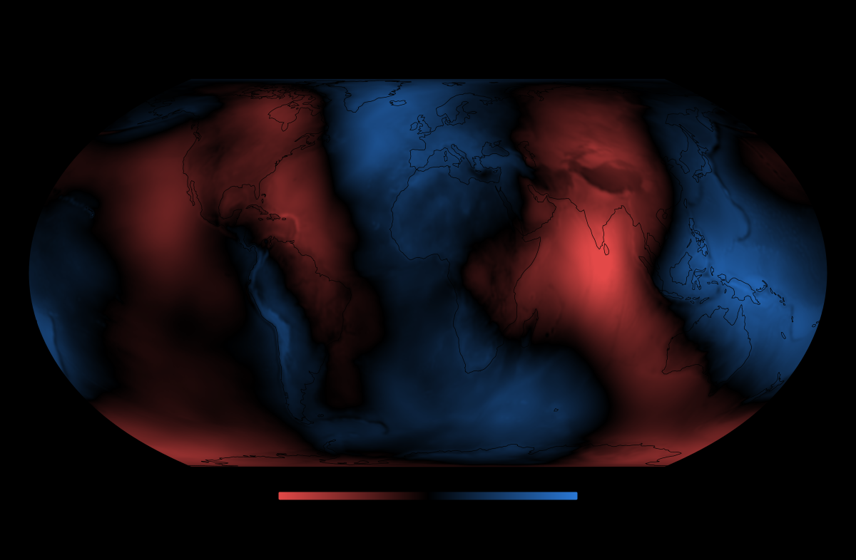
The geoid from GOCO06s, drawn with this crate.

Install

cargo add geopotential

Example: a field and what it does

use geopotential::{Coefficients, Functional};

// A field with a single term: J2, Earth's flattening.
let mut field = Coefficients::zeros(3.986004415e14, 6_378_136.3, 2);
field.set(2, 0, -4.84165e-4, 0.0);

// Geoid height at the equator and at the North Pole.
let lats = [0.0, 90f64.to_radians()];
let geoid = field.grid(&Functional::GeoidHeight, field.radius, &lats, &[0.0]);
assert!(geoid[0] > 0.0); // the equatorial bulge
assert!(geoid[1] < 0.0); // flatter at the poles

// Add the central term (C̄00 = 1) and find gravity on a satellite 400 km above northern Italy.
field.set(0, 0, 1.0, 0.0);
let r = 6_378_137.0 + 400e3;
let (lat, lon) = (45f64.to_radians(), 7f64.to_radians());
let [north, east, up] = field.partials(r, lat, lon).acceleration_neu(r, lat);
assert!(up < -8.0); // pointing down, about 8.7 m/s²
assert!(north.abs() > 0.0 && east == 0.0);

Example: read a real model

Download a model first, for example GOCO06s.gfc from the ICGEM model table.

use geopotential::{julian_epoch, read_gfc};

fn main() -> Result<(), Box<dyn std::error::Error>> {
    let gfc = read_gfc(&std::fs::read_to_string("GOCO06s.gfc")?)?;

    // Time-variable models apply their trends and annual terms; static ones ignore the date.
    let field = gfc.model.at(julian_epoch(2026, 7, 16, 12, 0));
    println!("{} to degree {}, C20 = {:e}", gfc.name.unwrap_or_default(), field.max_degree(), field.c(2, 0));
    Ok(())
}

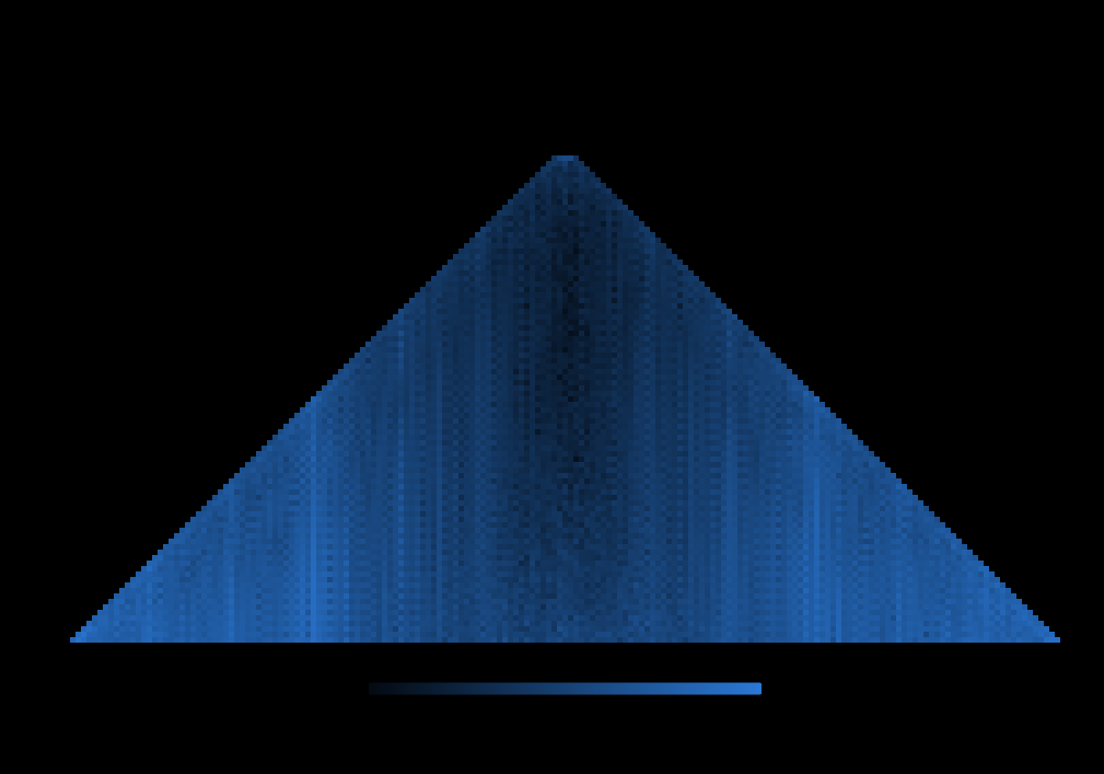
The calibrated error of each coefficient of the July 2026 COST-G field, read with read_gfc.

What is inside

Item	What it does
Legendre	Normalized Legendre functions and their derivatives, stable to degree 2700 at every latitude (Holmes & Featherstone 2002)
Coefficients	The coefficients with their GM, radius and tide system; degree variances, rescaling, truncation and tide-system conversion (IERS Conventions 2010, ch. 6)
TimeVariable	Models with trends and periodic terms, evaluated at any date (ICGEM)
partials, second_partials	Potential, gravity vector and gravity-gradient tensor at a point; the geopotential and gravity with the centrifugal term, and the deflections of the vertical
normal	The normal gravity of a level ellipsoid from its four defining constants: GRS80 and WGS84 as Somigliana’s formula on and above the ellipsoid, U₀, the zonal harmonics and the normal field as coefficients, Bruns’ formula with its zero-degree term, and dynamic and normal heights from geopotential numbers (Moritz 2000; Heiskanen & Moritz 1967)
grid with Functional	Maps of geoid height, gravity anomaly or disturbance, radial gradient or equivalent water height (Barthelmes 2013; Wahr et al. 1998)
Coefficients::analysis, gauss_grid, gauss_legendre	The exact inverse of grid: any functional on a Gauss–Legendre grid back to coefficients, by Gauss–Legendre quadrature
slepian	Slepian functions of a polar cap from Grünbaum’s commuting tridiagonal matrix, and of any region (a cap anywhere, a polygon) from its concentration matrix, integrated exactly in longitude and on clustered Gauss–Legendre panels in colatitude; the basin kernel that averages a field over a region, with the least leakage (Simons, Dahlen & Wieczorek 2006; Swenson & Wahr 2002)
read_gfc, Gfc	ICGEM .gfc models, static or time-variable (icgem1.0 and 2.0), with their errors (format)
julian_epoch, parse_date	The decimal-year dates these files use
bodies	Potential, attraction and gradient tensor of a uniform body in closed form: a rectangular prism (Nagy, Papp & Benedek 2000), finite on its faces and edges, with a Gauss–Legendre cubature of Bernstein-ellipse order outside it that holds 10⁻¹⁴ on needles and plates where the corner sums lose 10⁻⁸ (Fukushima 2019 diagnosed the loss); and a triangulated polyhedron (Werner & Scheeres 1997), whose trace is an inside test, with a mesh check and a cubature over its tetrahedra far away
planar	Level grids in the wavenumber domain: upward continuation, reduction to the pole (plain or Wiener-damped) and to the equator, any change of field direction, Baranov pseudo-gravity (Blakely 1995, ch. 12), or any kernel through Grid::filter, with edge padding and a cosine taper against the periodic wrap; and Euler deconvolution of a profile or a grid for a source’s position and the background, with its covariance, in moving windows, and as Euler inversion, which fits the data too and picks the structural index (Reid & Thurston 2014; Uieda et al. 2025)
special	Complete elliptic integrals K and E by the arithmetic–geometric mean; Bulirsch’s general complete integral cel (Bulirsch 1969); Carlson’s symmetric R_F, R_D, R_J, R_C with their principal values (Carlson 1995); Legendre’s incomplete F, E and Π for any m, with Π beyond its pole as a principal value (DLMF §19.25); and ring, the average of 1/r over a ring and its gradient, which rings of mass, charge and current share
linalg	Pivoted Gaussian elimination for general systems, Cholesky for the normal equations of least squares, and symmetric eigenproblems by Jacobi’s method or, for large matrices, Householder reduction and the implicit QL iteration
fft	The radix-2 fast Fourier transform, for time series, and fftn in any number of dimensions with wavenumber, for gridded fields

Conventions:

• angles in radians, geocentric latitude;
• fully normalized coefficients with no Condon–Shortley phase, as in ICGEM files;
• the optional serde feature serializes Coefficients.

Models are free from ICGEM; each COST-G monthly series also comes as one zip.

Applications

• Height systems. Turning a GNSS ellipsoidal height into a usable one needs the geoid; this is the synthesis behind national models such as GEOID2022 and AUSGeoid2020, and normal turns a levelled geopotential number into a dynamic or normal height.
• Orbit design and determination. J2 from a real model sets the nodal precession that makes an orbit sun-synchronous; examples/sun_synchronous_orbit.rs reproduces Landsat’s 98.2°.
• Inertial navigation. The deflection of the vertical is what an accelerometer mistakes for horizontal acceleration, and compensating it from a model is standard practice.
• Gradiometry. SecondPartials::tensor_neu gives the tidal tensor a gradiometer measures, in which a vehicle’s own acceleration cancels.
• Reading published models. read_gfc takes any ICGEM .gfc file, static or time-variable.

How it is checked

• Legendre functions: against closed forms, the addition theorem to degree 2700 close to the pole, and the Legendre equation.
• Derivatives: against finite differences.
• The field: against Laplace’s equation, and the IERS tide offset of C̄20.
• An independent implementation: the degree-300 GOCO06s model agreed with the former geo5d crate’s synthesis to about 1e-15.
• Normal gravity: every derived constant that Moritz (2000) prints for GRS80 and the WGS84 document prints for WGS84 (γ_e, γ_p, k, U₀, J₂–J₈, the even zonals), to their digits; the synthesized normal field is Somigliana’s gravity to 10⁻¹⁰ m/s²; the free-air gradient 0.3086 mGal/m.
• Bodies: Fukushima’s (2019) Table 4 prism to 10⁻¹⁴; a 1×1×100 needle and a 100×100×1 plate to 3×10⁻¹⁴ from 0.3 off their sides to 100 Brillouin radii; a cube mesh against the prism across the polyhedron’s hand-over and out to 1000 sizes; a dented, non-convex mesh.
• Special functions: Carlson’s check values and principal values; Abramowitz & Stegun’s Tables 17.5, 17.6 and 17.9 within their rounding, DLMF’s special values and periods, Π beyond its pole against DLMF 19.25.16.
• Planar: padding against the periodic wrap; reduction to the equator at 10° inclination to 1%; Euler deconvolution exact for a dipole, a point mass and a line mass, and Euler inversion’s misfit picking the structural index.
• Slepian functions: a cap away from the pole has the polar cap’s spectrum to 10⁻¹²; a box and a triangle have their exact areas and Shannon numbers; the basin mean of P̄₂₀ over a cap in closed form.
• Real files from COST-G and GOCO06s, which bend the format in practice: missing header markers, comment and warning lines, errors empirical, and free text before the header. A malformed record fails with its line number. The fixtures’ sources are listed in tests/data/README.md.

One of eight crates in physica: physica (all of them, plus cross-domain analogies) · metrology (constants) · geopotential (the gravity field) · gravimetry (missions and GRACE) · gravitational (waves) · gravitics (frontier gravity) · magnetics (magnetism and MHD) · plasmoid (fusion plasma).

Modules

bodies

The Newtonian potential of uniform bodies, in closed form: what a survey’s forward model sums over a grid of prisms, or over the triangles of an asteroid’s shape model.

fft

The fast Fourier transform, for gridded fields and time series alike.

linalg

Dense linear algebra that the potential-field crates share: pivoted Gaussian elimination for a general system, and Cholesky for the symmetric positive-definite normal equations of least squares.

normal

The normal gravity field: the gravity of a level ellipsoid of revolution, the reference that gravity anomalies, geoid heights and physical heights are measured against.

planar

Potential fields on a level grid, in the wavenumber domain: upward continuation, reduction to the pole and pseudo-gravity (Blakely, Potential Theory in Gravity and Magnetic Applications, 1995, ch. 12).

slepian

Slepian functions: the bandlimited functions on the sphere best concentrated inside a region (Simons, Dahlen & Wieczorek, SIAM Rev. 48, 504, 2006). They are the basis for averaging a gravity field over a basin, or a magnetic field over a region, with the least leakage from outside it.

special

Special functions that potential fields share: the elliptic integrals of rings of mass, charge and current, and the ring itself.

Structs

Coefficients

A spherical-harmonic gravity field: fully normalized (4π, no Condon–Shortley phase) Stokes coefficients C̄nm, S̄nm up to a maximum degree, with the GM and reference radius they belong to.

Gfc

A parsed .gfc file.

Legendre

A reusable table of P̄nm (and optionally ∂P̄nm/∂φ) for all 0 ≤ m ≤ n ≤ nmax at one latitude. The recursion coefficients are computed once in Legendre::new.

Partials

The gravitational potential and its first partial derivatives at one point.

SecondPartials

The potential with its first and second partial derivatives in (r, φ, λ) at one point: what a gravity-gradient tensor is built from.

Term

One time-variable record of coefficient (n, m). All times are decimal years.

TimeVariable

A time-variable model as ICGEM defines it (e.g. GOCO06s, EIGEN-6S4): G(t) = G(t0) + trnd·(t−t0) + Σ_k [asin_k·sin(2π(t−t0)/p_k) + acos_k·cos(2π(t−t0)/p_k)].

Enums

Functional

A quantity that is a per-degree multiple of the harmonic sum Σ_m P̄nm(sin φ)(C̄nm cos mλ + S̄nm sin mλ) (spherical approximation).

GfcError

Why a .gfc file could not be read. Line numbers are 1-based.

TermKind

What a time-variable ICGEM record contributes to a coefficient at time t.

TideSystem

How the permanent tide is treated in C̄20.

Constants

MAX_DEGREE

Highest degree the scaled recursion supports before P̄nm / cos^m φ can overflow near the poles (Holmes & Featherstone 2002).

RHO_EARTH

Mean density of the Earth used by Wahr et al. (1998), kg/m³. gravity-toolkit instead derives it from GM (≈5.51e3), which changes water heights by about 0.1%.

RHO_WATER

Density of fresh water, kg/m³.

Traits

Field

A static field with a scalar potential V, evaluated at geocentric radius r (m), latitude lat and longitude lon (radians).

Functions

gauss_grid

The grid that Coefficients::analysis reads to degree nmax: nmax + 1 Gauss–Legendre latitudes (radians, south to north) and 2·nmax + 2 longitudes 2πj/(2·nmax + 2).

gauss_legendre

The n nodes (ascending) and weights of Gauss–Legendre quadrature on [−1, 1], exact for polynomials of degree up to 2n − 1: Newton’s method on P_n from Tricomi’s starting values, with the weights 2/((1 − x²)P_n′²) and the symmetry about 0 imposed.

geocentric

Geocentric radius (m) and latitude (radians) of a point at geodetic latitude lat (radians) and height height (m) above the WGS84 ellipsoid: where to evaluate a Field for a point given by GNSS or a map. NormalGravity::geocentric does the same for any ellipsoid.

julian_epoch

The Julian epoch (years of 365.25 days from J2000.0, TT ignored) of a calendar date and time. ICGEM time-variable terms use (t − t0) in these years: GOCO06s defines its annual period as 365.25 d.

parse_date

Parse yyyymmdd or yyyymmdd.hhmm into a Julian epoch.

read_gfc

Read an ICGEM .gfc file.