library(scales)
library(tidyverse)
library(readr)
is_highwayhash <- Vectorize(function(fn) {
switch(fn,
"avx" = TRUE,
"sse" = TRUE,
"portable" = TRUE,
FALSE)
})
get_line_type <- Vectorize(function(fn) {
switch(fn,
"avx" = "highwayhash",
"sse" = "highwayhash",
"portable" = "highwayhash",
"other")
})
df <- read_csv("./highway.csv")
df <- mutate(df,
fn = `function`,
highwayhash = is_highwayhash(fn),
line = get_line_type(fn),
throughput = value * iteration_count * 10^9 / sample_time_nanos) %>%
filter(group != 'highway-builder')
pal <- hue_pal()(df %>% select(fn) %>% distinct() %>% count() %>% pull())
names(pal) <- df %>% select(fn) %>% distinct() %>% pull()
df64 <- df %>% filter(group == '64bit')
df256 <- df %>% filter(group == '256bit')
byte_rate <- function(l) {
paste(scales::number_bytes(l, symbol = "GB", units = "si"), "/s")
}
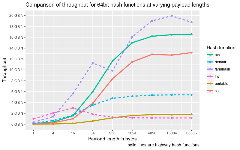
ggplot(df64, aes(value, throughput, color = fn)) +
stat_summary(fun.y = mean, geom="point", size = 1.5) +
stat_summary(aes(linetype = line), fun.y = mean, geom="line", size = 1.2) +
scale_y_continuous(labels = byte_rate, limits = c(0, NA), breaks = pretty_breaks(10)) +
scale_x_continuous(trans='log2', limit = c(1, NA), breaks = c(1, 4, 16, 64, 256, 1024, 4096, 16384, 65536)) +
labs(title = "Comparison of throughput for 64bit hash functions at varying payload lengths",
caption = "solid lines are highway hash functions",
col = "Hash function",
y = "Throughput",
x = "Payload length in bytes") +
guides(linetype = FALSE) +
scale_colour_manual( values = pal)
ggsave('64bit-highwayhash.png', width = 8, height = 5, dpi = 100)
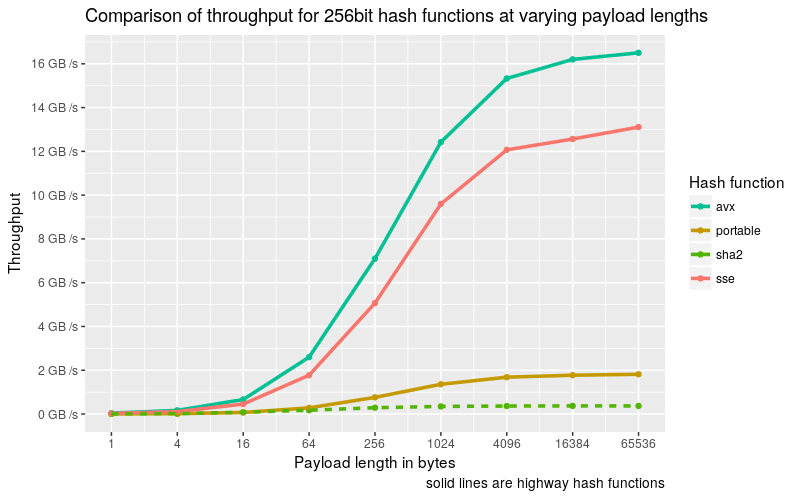
ggplot(df256, aes(value, throughput, color = fn)) +
stat_summary(fun.y = mean, geom="point", size = 1.5) +
stat_summary(aes(linetype = line), fun.y = mean, geom="line", size = 1.2) +
scale_y_continuous(labels = byte_rate, limits = c(0, NA), breaks = pretty_breaks(10)) +
scale_x_continuous(trans='log2', limit = c(1, NA), breaks = c(1, 4, 16, 64, 256, 1024, 4096, 16384, 65536)) +
labs(title = "Comparison of throughput for 256bit hash functions at varying payload lengths",
caption = "solid lines are highway hash functions",
col = "Hash function",
y = "Throughput",
x = "Payload length in bytes") +
guides(linetype = FALSE) +
scale_colour_manual(values = pal)
ggsave('256bit-highwayhash.png', width = 8, height = 5, dpi = 100)
ggplot(df %>% filter(highwayhash == TRUE), aes(value, throughput, color = fn, line_type = group)) +
stat_summary(fun.y = mean, geom="point", size = 1.5) +
stat_summary(aes(linetype = as.factor(group)), fun.y = mean, geom="line", size = 1.2) +
scale_y_continuous(labels = byte_rate, limits = c(0, NA), breaks = pretty_breaks(10)) +
scale_x_continuous(trans='log2', limit = c(1, NA), breaks = c(1, 4, 16, 64, 256, 1024, 4096, 16384, 65536)) +
labs(title = "Comparison of throughput for 64bit vs 256bit highway hash",
caption = "solid lines are 256bit",
col = "Hash function",
y = "Throughput",
x = "Payload length in bytes") +
guides(linetype = FALSE) +
scale_colour_manual(values = pal)
ggsave('64bit-vs-256it-highwayhash.png', width = 8, height = 5, dpi = 100)
reldf <- df %>%
mutate(throughput = throughput / 10^9) %>%
group_by(group, fn, highwayhash, value) %>%
summarize(throughput = mean(throughput)) %>%
ungroup() %>%
group_by(value) %>%
mutate(relative = throughput / max(throughput)) %>%
ungroup() %>%
complete(group, fn, value, fill = list(highwayhash = FALSE))
ordered <- reldf %>% distinct(fn, highwayhash) %>% arrange(highwayhash, fn) %>% pull(fn)
reldf$fn <- factor(reldf$fn, levels = ordered)
ggplot(reldf, aes(fn, as.factor(value))) +
geom_tile(aes(fill = relative), color = "white") +
facet_grid(group ~ .) +
scale_x_discrete(position = "top") +
scale_fill_gradient(name = "", low = "white", high = "steelblue", na.value = "#D8D8D8", labels = c("lowest", "highest (GB/s)"), breaks = c(0,1)) +
xlab("Hash Library") +
ylab("Payload Size (bytes)") +
geom_text(size = 3.25, aes(label = ifelse(is.na(relative), "NA", format(round(throughput, 2), digits = 3)))) +
theme(axis.text.x.top=element_text(angle=45, hjust=0, vjust=0)) +
theme(legend.position="bottom") +
theme(plot.caption = element_text(hjust=0)) +
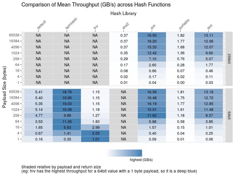
ggtitle("Comparison of Mean Throughput (GB/s) across Hash Functions") +
labs(caption = "Shaded relative by payload and return size\n(eg: fnv has the highest throughput for a 64bit value with a 1 byte payload, so it is a deep blue)")
ggsave('highwayhash-table.png', width = 8, height = 6, dpi = 100)