Crate arael

Expand description

ARAEL – Algorithms for Robust Autonomy, Estimation, and Localization.

Nonlinear optimization framework with compile-time symbolic differentiation.

Define model structs with optimizable parameters, write constraints as symbolic expressions, and the framework symbolically differentiates at compile time, applies common subexpression elimination, and generates compiled cost, gradient, and Gauss-Newton hessian (J^T J approximation) code.

§Features

Symbolic math – expression trees with automatic differentiation, simplification, LaTeX/Rust code generation (via arael-sym)
Compile-time constraint code generation – write constraints symbolically, get compiled derivative code with CSE
Levenberg-Marquardt solver – with robust error suppression via the Starship method (US12346118) gamma * atan(r / gamma) and switchable constraints (guard = expr)
Multiple solver backends via LmSolver trait:
- Dense Cholesky (nalgebra) – fixed-size dispatch up to 9x9
- Band Cholesky – pure Rust O(n*kd^2) for block-tridiagonal systems
- Sparse Cholesky (faer, pure Rust) – for general sparse hessians
- Eigen SimplicialLLT and CHOLMOD (SuiteSparse) – optional C++ backends via FFI
- LAPACK band – optional dpbsv/spbsv backend
Indexed sparse assembly – precomputed position lists for zero-overhead hessian assembly after first iteration
f32 and f64 precision – #[arael(root)] for f64, #[arael(root, f32)] for f32 throughout
Model trait – hierarchical serialize/deserialize/update protocol
Type-safe references – Ref<T>, Vec<T>, Deque<T>, Arena<T>
Runtime differentiation – parse equations from strings at runtime, auto-differentiate symbolically, and optimize via ExtendedModel + TripletBlock (see examples/runtime_fit_demo.rs)
Hessian blocks – SelfBlock<A> and CrossBlock<A, B> for 1- and 2-entity constraints (packed dense); TripletBlock for 3+ entities (COO sparse)
Jacobian computation – #[arael(root, jacobian)] generates calc_jacobian() returning a sparse Jacobian<T> matrix for DOF analysis via SVD. #[arael(constraint_index)] tracks constraint provenance per row. See examples/jacobian_demo.rs.
Gimbal-lock-free rotations – EulerAngleParam optimizes a small delta around a reference rotation matrix
WASM/browser support – compiles to WebAssembly; the arael-sketch constraint editor runs in the browser via eframe/egui

§Scope

Arael is a nonlinear optimization framework, not a complete SLAM or state estimation system. The SLAM and localization demos show how to use arael as the optimizer backend, but a production SLAM pipeline would additionally need:

Front-end perception: feature detection, descriptor extraction
Data association: matching observed features to existing landmarks, handling ambiguous or incorrect matches
Landmark management: initializing new landmarks from observations, merging duplicates, pruning unreliable ones
Keyframe selection: deciding when to add new poses vs. discard redundant frames
Loop closure: detecting revisited places, verifying loop closure candidates, and injecting constraints
Outlier rejection logic: deciding which observations to reject
Marginalization / sliding window: limiting optimization scope for real-time operation, marginalizing old poses while preserving their information
Map management: spatial indexing, map saving/loading, multi-session map merging

Arael provides the compile-time-differentiated solver that sits at the core of such a system. Everything above is application-level logic that builds on top of it.

§Example: Symbolic Math

use arael::sym::*;

arael::sym! {
    let x = symbol("x");
    let f = sin(x) * x + 1.0;

    println!("f(x)   = {}", f);           // sin(x) * x + 1
    println!("f'(x)  = {}", f.diff("x")); // x * cos(x) + sin(x)

    let vars = std::collections::HashMap::from([("x", 2.0)]);
    println!("f(2.0) = {}", f.eval(&vars).unwrap()); // 2.8185...
}

The sym! macro auto-inserts .clone() on variable reuse, so you write natural math without ownership boilerplate. See docs/SYM.md for the full symbolic math reference.

§Example: Robust Linear Regression

Define a model with optimizable parameters and a residual expression. The Starship method gamma * atan(plain_r / gamma) suppresses outlier influence while preserving smooth differentiability:

#[arael::model]
struct DataEntry { x: f32, y: f32 }

#[arael::model]
#[arael(fit(data, |e| {
    let plain_r = (a * e.x + b - e.y) / sigma;
    gamma * atan(plain_r / gamma)
}))]
struct LinearModel {
    a: Param<f32>,
    b: Param<f32>,
    data: Vec<DataEntry>,
    sigma: f32,
    gamma: f32,
}

The macro generates calc_cost(), calc_grad_hessian(), and fit() with symbolically differentiated, CSE-optimized compiled code. The robust fit ignores outliers while tracking the inlier data:

Linear Regression

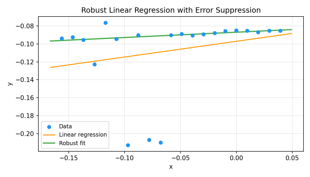
See examples/linear_demo.rs for the full source.

§Runtime Differentiation

Compile-time differentiation generates optimized Rust code with CSE at build time – ideal when the model structure is fixed. But many applications need equations that are only known at runtime: user-typed formulas in a CAD parametric dimension, configuration-driven curve fitting, or symbolic constraints loaded from a file.

Arael supports this through runtime differentiation: parse an equation string with arael_sym::parse, symbolically differentiate once at setup with E::diff, then evaluate the expression tree numerically each solver iteration. The ExtendedModel trait and TripletBlock provide the integration point with the LM solver.

The sketch editor (arael-sketch) uses this extensively for parametric expression dimensions – a user can type d0 * 2 + 3 as a dimension value, and the solver constrains the geometry to satisfy the equation in real time, with full symbolic derivatives.

The model uses #[arael(root, extended)] and implements ExtendedModel to push residuals and derivatives into a TripletBlock at each solver iteration:

#[arael::model]
#[arael(root, extended)]
struct RegressionModel {
    coeffs: refs::Vec<Coefficient>,         // optimizable parameters
    hb: TripletBlock<f64>,                  // Gauss-Newton accumulator
    residual_expr: Option<arael_sym::E>,    // parsed equation
    derivs: Vec<(String, u32, arael_sym::E)>, // pre-computed derivatives
    // ...
}

impl ExtendedModel for RegressionModel {
    fn extended_compute64(&mut self, params: &[f64], grad: &mut [f64]) {
        for &(x, y) in &self.data {
            vars.insert("x", x);
            vars.insert("y", y);
            let r = residual.eval(&vars).unwrap();
            let dr: Vec<f64> = self.derivs.iter()
                .map(|(_, _, d)| d.eval(&vars).unwrap()).collect();
            // writes 2*r*dr into grad AND pushes full upper-triangle
            // Hessian into the TripletBlock (one call, both done)
            self.hb.add_residual(r, &indices, &dr, grad);
        }
    }
}

See examples/runtime_fit_demo.rs for a complete example that accepts an arbitrary equation from the command line and fits it to data with robust error suppression.

§Model Structure

This is the reference for every piece that appears in an #[arael::model] declaration: parameter types, Hessian blocks, collection types, macro attributes, and the patterns for placing constraints. For end-to-end code, see examples/single_root_demo.rs (smallest complete model) and examples/slam_demo.rs (full SLAM setup). A markdown mirror lives at docs/MODEL.md.

§Parameter types

Type	Size	Use it when
`Param<f32>` / `Param<f64>`	1	scalar parameter
`Param<vect2<T>>`	2	2D point / direction
`Param<vect3<T>>`	3	3D position, velocity, linear vector
`SimpleEulerAngleParam<T>`	3	three direct Euler angles (roll, pitch, yaw)
`EulerAngleParam<T>`	3	“universal” delta composed with a fixed reference rotation; avoids parameterisation singularities for large-angle motion

#[arael::model]
struct Pose {
    pos: Param<vect3f>,              // 3 scalar params
    ea: SimpleEulerAngleParam<f32>,  // 3 scalar params (roll, pitch, yaw)
    // info: plain non-Param data (sigmas, measurements) is fine
    info: PoseInfo,
    hb_pose: SelfBlock<Pose, f32>,   // mandatory; see below
}

Every parameter stores a current value and a per-iteration work() copy. The macro rewrites pose.ea in a constraint body to pose.ea.work() so the LM trial step is evaluated without mutating the stored value until the step is accepted.

§Initial values via the `_value` suffix

Inside a constraint body, pose.pos_value (any <field>_value) resolves to the original stored value of the parameter – the point the LM trial-step is measured against, not the trial step itself. Use it to build drift / regularising residuals:

let pos_drift = pose.pos - pose.pos_value;
[pos_drift.x * path.drift_pos_isigma,
 pos_drift.y * path.drift_pos_isigma,
 pos_drift.z * path.drift_pos_isigma]

§Parameter control

Three ways to keep a parameter out of the solve:

Param::fixed(v) at construction – immutable; the macro never emits indices for it. Typical use: problem-wide constants that happen to be parameter-shaped (e.g. a known camera pose).
Mutate .optimize at runtime – pose.pos.optimize = false; freezes a live parameter for the next solve call. Flip it back on to re-include. Use for staged optimisation (freeze subset, solve, unfreeze, solve again).
The _value trick above – the parameter still moves but the residual is anchored to its initial position via a drift constraint.

// (1) fixed at construction
let camera = Pose {
    pos: Param::fixed(known_position),     // never optimised
    ea:  Param::fixed(known_orientation),
    /* ... */
};

// (2) runtime freeze for a staged solve
for pose in path.poses.iter_mut() {
    pose.pos.optimize = false;
    pose.ea.optimize = false;
}
// ...solve only the remaining live params...
for pose in path.poses.iter_mut() {
    pose.pos.optimize = true;
    pose.ea.optimize = true;
}

See Path::optimise_center in loc_global_demo.rs for a real usage of runtime .optimize = false – it freezes every pose, solves only for the root-level global rigid transform, bakes the result into the poses, then un-freezes.

§Hessian block types

The full Gauss-Newton Hessian is a symmetric block matrix, with one block per (entity, entity) pair in the parameter vector. The block at position (Ei, Ej) is the NEi × NEj matrix of second partials; by symmetry H[Ei, Ej] = H[Ej, Ei]^T. arael stores each unique block once and lets the accumulator fill in the transpose when assembling into a dense / band / sparse matrix. Every constraint that couples a given pair adds its 2 * dr_i * dr_j contribution to the same block:

Diagonal blocks (Ei == Ej) live in each entity’s SelfBlock<Ei> and are symmetric; only the upper triangle is stored. Every constraint touching Ei’s params writes there additively.
Off-diagonal blocks (Ei != Ej) live in a CrossBlock<Ei, Ej> or in a TripletBlock that covers the pair. One CrossBlock<A, B> covers both H[A, B] and its transpose H[B, A] – the accumulator writes both halves from the single stored rectangle.

Gradient contributions 2 * r * dr go directly into the LM- provided global gradient slice – not into any block. Only Hessian entries are stored block-wise.

Pick the block shape that matches the constraint body’s parameter reach:

Type	Stores	Pick it when
`SelfBlock<T>`	grad + upper-triangular Hessian for entity T’s own params	mandatory on every params-having struct. Holds the per-entity gradient and the (T, T) block
`CrossBlock<A, B>`	rectangular (A, B) cross Hessian only	default for cross-entity Hessian pairs. Packed in-place writes, cheap to assemble. One per unordered (A, B) entity pair; (A, A) / (B, B) diagonals stay on each entity’s `SelfBlock`
`TripletBlock<T>`	COO across-entity pairs	always placed on the root (one `hbt: TripletBlock<T>` on the root struct; constraints reach it via the `root.<field>` block spec). Two canonical uses: (1) the root has its own `Param` fields and constraints couple entity params with root params – the (entity, root) cross pair lives in the root’s TripletBlock; (2) runtime-parsed residuals via `ExtendedModel` that can’t enumerate per-pair CrossBlocks statically – `extended_compute` writes into the root’s TripletBlock directly. Never on a non-root struct. Noticeably slower to assemble* – every entry is a `Vec` push

SelfBlock<Self> is required on every Model that has parameters – omitting it is a compile-time error. Grad and diagonal writes always land on each entity’s SelfBlock; CrossBlock and TripletBlock are cross-only storage.

// Entity with its mandatory SelfBlock.
#[arael::model]
struct Pose {
    pos: Param<vect3f>,
    ea:  SimpleEulerAngleParam<f32>,
    hb_pose: SelfBlock<Pose, f32>,   // required
}

// Constraint struct linking two entities via a CrossBlock.
#[arael::model]
#[arael(constraint(hb, { /* residuals involving prev and cur */ }))]
struct PosePair {
    #[arael(ref = root.poses)] prev: Ref<Pose>,
    #[arael(ref = root.poses)] cur:  Ref<Pose>,
    hb: CrossBlock<Pose, Pose, f32>, // only the (prev, cur) cross block
}

§Multi-CrossBlock vs TripletBlock

For N-entity residuals the macro accepts two shapes:

constraint([hb_ab, hb_ac, hb_bc], { ... }) – one CrossBlock<A, B> field per unordered entity pair on the constraint struct. Packed rectangular storage, one add_residual_cross per pair.
constraint(..., root.hbt, { ... }) – route across-entity pairs into a root-owned TripletBlock<T>. One COO accumulator on the root absorbs cross pairs from every constraint that references it. The TripletBlock always lives on the root – don’t put one on a constraint struct or an entity struct; the macro’s root.<field> block spec is the only correct way to reach a TripletBlock.

Prefer multi-CrossBlock whenever the set of cross-pairs is fixed and dense. TripletBlock carries a significant Hessian-assembly penalty: every cross entry is a Vec<(u32, u32, T)> push (with growth and no locality), whereas CrossBlock writes in place into a pre-sized NA * NB rectangle at a known offset. The same N-entity constraint assembles substantially faster through multi-CrossBlock, and the rectangular layout is friendlier to the CSC factorisation that follows.

Reach for the root-owned TripletBlock in two canonical situations:

The root has its own Param fields and constraints couple per-entity params with root params. The (entity, root) cross pair has to live somewhere; a dedicated CrossBlock<Entity, Root> per entity type is verbose and scatters the cross storage, so the root TripletBlock is the clean place for it. The loc_global_demo example uses this – hbt: TripletBlock<f32> on Path absorbs every pose-to-globals cross pair emitted by the tilt and related constraints.
Runtime-parsed residuals via ExtendedModel. When the residual body is a user-supplied expression parsed at runtime, the macro cannot enumerate per-pair CrossBlocks statically. ExtendedModel::extended_compute* writes directly into the root’s TripletBlock instead – see examples/runtime_fit_demo.rs.

In both cases the triplet lives on the root, not on a constraint struct.

Caveat for case 1 – root-level Params destroy sparsity. Every constraint that reads a root param introduces an (entity, root) cross pair in the Hessian. If many constraints read the same root param – which is the whole point of “global” root params – the root’s rows and columns in the Hessian become dense (coupled to every entity that touches them). Sparse Cholesky’s fill-in grows accordingly and solve times suffer. Use root Params only when the quantity is genuinely system-wide. Two canonical examples:

Frame corrections – rigid translation + rotation applied to every pose (the loc_global_demo pattern).
Global calibration – one-per-sensor quantities referenced by every observation from that sensor: camera intrinsics (fx, fy, cx, cy), lens-distortion coefficients, IMU bias and scale factors, magnetometer declination, barometric altitude reference. These live on the root naturally because there’s one of them for the whole problem and every measurement reads them.

Prefer per-entity params whenever the quantity is local. A root Param referenced by 1% of constraints is fine; one referenced by 90% of them will dominate factorisation cost.

// Multi-CrossBlock: explicit Hessian pair per unordered entity pair.
#[arael::model]
#[arael(constraint([hb_ab, hb_ac, hb_bc], { /* 3-line residual */ }))]
struct SymmetryLL {
    #[arael(ref = root.lines)] a: Ref<Line>,
    #[arael(ref = root.lines)] b: Ref<Line>,
    #[arael(ref = root.lines)] c: Ref<Line>,
    #[arael(cross = (a, b))] hb_ab: CrossBlock<Line, Line>,
    #[arael(cross = (a, c))] hb_ac: CrossBlock<Line, Line>,
    #[arael(cross = (b, c))] hb_bc: CrossBlock<Line, Line>,
}

// Root-owned TripletBlock: one COO accumulator on the root,
// referenced by constraints that couple an entity with root
// params (or where a per-pair CrossBlock layout doesn't fit).
#[arael::model]
#[arael(root)]
struct Path {
    poses: refs::Deque<Pose>,
    /* ... */
    hb:  SelfBlock<Path, f32>,
    hbt: TripletBlock<f32>,   // shared across-entity accumulator
}

#[arael(constraint([hb_pose, root.hbt], { /* residual touching pose + root */ }))]
struct Pose { /* ... hb_pose: SelfBlock<Pose, f32> ... */ }

§Collection types

Type	Use it when
`refs::Vec<T>`	dense indexed list, contiguous storage, stable `Ref<T>` handles
`refs::Deque<T>`	like `Vec` but supports `push_front` / `push_back` (rolling pose history)
`refs::Arena<T>`	arbitrary insertion / deletion with stable handles
`Ref<T>`	a handle into the containing collection

A Model struct is “directly composed” when a child Model appears as a plain field (e.g. sub: Sub in single_root_demo.rs). It’s “collection-composed” when wrapped in one of the containers above.

#[arael::model]
#[arael(root)]
struct Path {
    // collection-composed: many Pose instances, iterated by the macro
    poses: refs::Deque<Pose>,
    // direct composition: a single Sub entity as a plain field
    globals: Globals,
    hb: SelfBlock<Path, f64>,
}

§Struct-level macro attributes

Attribute	Purpose
`#[arael::model]`	declare a Model; generates Model trait impl
`#[arael(root)]`	mark the top-level Model. Generates `LmProblem` impl, manages indices, owns the update cycle
`#[arael(root, f32)]`	scalar precision for the generated solver surface (default is f64)
`#[arael(root, jacobian)]`	additionally emit `calc_jacobian` and `calc_cost_table` for diagnostics
`#[arael(root, fit(coll, \|e\| body))]`	shorthand: sum-of-squares fit of a residual body over one collection
`#[arael(skip_self_block)]`	opt out of the mandatory `SelfBlock<Self>` (rare)

Constraints can also appear on the root itself – useful for regularising root-level parameters.

// Root-level constraint pinning global_delta near its initial value.
#[arael::model]
#[arael(root, f32, jacobian)]
#[arael(constraint(hb, name = "global_delta_drift", {
    let d = path.global_delta - path.global_delta_value;
    [d.x * path.drift_pos_isigma,
     d.y * path.drift_pos_isigma,
     d.z * path.drift_pos_isigma]
}))]
struct Path {
    // ...
    global_delta: Param<vect3f>,
    drift_pos_isigma: f32,
    hb: SelfBlock<Path, f32>,
}

§Constraint attributes

Block-spec forms:

#[arael(constraint(hb, { body }))]                      // single local block
#[arael(constraint([hb_ab, hb_ac, hb_bc], { body }))]   // bracketed multi-block (N ≥ 2)
#[arael(constraint(pose.hb_pose, { body }))]            // remote SelfBlock via Ref field
#[arael(constraint(hb_pose, root.hbt, { body }))]       // self-primary + root-owned TripletBlock

N ≥ 2 block lists must use the bracketed form. The only exception is the specific 2-item positional shape constraint(<local_self_block>, root.<triplet>, { body }) above, which carries distinct semantics (self-primary routing across the entity / root cross-pair). Writing constraint(hb_a, hb_b, hb_c, { body }) is rejected at macro expansion – use constraint([hb_a, hb_b, hb_c], { body }).

Dotted names mean two different things depending on the first segment:

<ref_field>.<block> – reach through a Ref<T> field on this struct to the target entity’s SelfBlock. PointFrine uses this to write grad / diagonal into the referenced Pose.
root.<triplet> – the literal keyword root points at a TripletBlock field on the root struct. Cross pairs between this entity’s params and root’s params route into that TripletBlock in COO.

// Remote SelfBlock: PointFrine lives on PointLandmark but writes
// pose's diagonal via pose.hb_pose; the (pose, path) cross-pair
// goes into a local CrossBlock<Pose, Path>.
#[arael::model]
#[arael(constraint([pose.hb_pose, hb_root], parent = lm, {
    /* residual involving lm, pose, feature, path */
}))]
struct PointFrine {
    #[arael(ref = root.poses)]         pose:    Ref<Pose>,
    #[arael(ref = pose.info.features)] feature: Ref<PointFeature>,
    hb_root: CrossBlock<Pose, Path, f32>,
}

// Self-primary + root-owned TripletBlock: tilt on Pose references
// path.global_rot, so the pose<->path cross pair needs somewhere
// to live. `root.hbt` names a TripletBlock field on the Path root.
#[arael(constraint(hb_pose, root.hbt, {
    let mr_global = path.global_rot.rotation_matrix();
    let mr2w_eff  = mr_global * pose.ea.rotation_matrix();
    let ea_eff    = mr2w_eff.get_euler_angles();
    [(ea_eff.x - pose.info.tilt_roll)  * path.tilt_isigma,
     (ea_eff.y - pose.info.tilt_pitch) * path.tilt_isigma]
}))]
struct Pose { /* ... hb_pose: SelfBlock<Pose, f32> ... */ }

Modifiers (comma-separated before the body):

Modifier	Purpose
`parent = <name>`	bind the parent iteration variable to `<name>` (default is `a_type.to_lowercase()`)
`name = "label"`	label the residual group. Shows up in `calc_cost_table` and `JacobianRow::label`
`guard = <bool expr>`	evaluated once per iteration; when false the whole constraint is skipped for that iteration
`<var>: <Type>`	declare an extra typed binding for the body

// `parent = lm` so the body can refer to the enclosing PointLandmark
// as `lm`; `name = "feature_obs"` labels the residual group; `guard`
// skips the whole constraint when the flag is false.
#[arael(constraint([pose.hb_pose, hb_root],
    parent = lm,
    name = "feature_obs",
    guard = feature.enabled,
    {
        /* residual using lm.pos, pose.*, feature.*, path.* */
    }
))]
struct PointFrine { /* ... */ }

Placement decides iteration:

Attribute on	What iterates	Typical use
Entity struct (`Pose`)	root iterates the containing collection	per-entity drift / tilt
Dedicated constraint struct (`PointFrine`) with `Ref<T>` fields	root iterates (often nested) collection of constraint structs	observation linking two or more entities
Root struct	fires once per solve	regularise root-level params, fix global DOF

§Field-level macro attributes

Attribute	Applies to	Purpose
`#[arael(ref = <path>)]`	`Ref<T>` field	where to resolve the Ref. `root.<collection>` or `<other_ref>.<sub_collection>`
`#[arael(cross = (<refA>, <refB>))]`	`CrossBlock<T, T>` field	disambiguate which ref pair a same-typed CrossBlock serves
`#[arael(constraint_index)]`	`u32` field	receives a unique row id per constraint instance; useful for diagnostics
`#[arael(skip)]`	any field	exclude from the Model’s serialize / accumulate paths (rare)

#[arael::model]
struct PointFeature {
    pixel: vect2f,
    // Camera is a Ref<Camera>; we don't want the macro to walk it
    // as a nested Model, so skip it.
    #[arael(skip)] camera: Ref<Camera>,
    // ... measurement data ...
}

#[arael::model]
#[arael(constraint(hb, { /* ... */ }))]
struct PosePair {
    #[arael(ref = root.poses)] prev: Ref<Pose>,
    #[arael(ref = root.poses)] cur:  Ref<Pose>,
    // constraint_index: the macro writes the per-constraint row id
    // here so you can correlate log entries to this specific pair.
    #[arael(constraint_index)] ci: u32,
    hb: CrossBlock<Pose, Pose, f32>,
}

§User-defined functions (`#[arael::function]`)

Constraint bodies have a fixed set of built-in ops (arithmetic, sin / cos / exp / sqrt / clamp / safe_asin / …, vector helpers). When your residual needs a custom function – a factored-out symbolic helper, or an opaque numerical routine with a known closed-form derivative – declare it with #[arael::function] and use it in constraint bodies the same way you’d use sin.

Two forms, distinguished by the attributed fn’s signature.

§Form A: purely symbolic

fn name(x: E, ...) -> E { expr } – the body is an arael-sym expression. The macro captures the body as an arael-sym source string, re-parses it at constraint-expansion time, and inlines the resulting E tree into the surrounding residual. Derivatives come from arael-sym’s own auto-diff.

use arael_sym::E;

#[arael::function]
fn sigmoid(x: E) -> E {
    1.0 / (1.0 + exp(-x))
}

#[arael::function]
fn square(x: E) -> E { x * x }

#[arael::model]
#[arael(root, jacobian)]
#[arael(constraint(hb, name = "fit", {
    [(sigmoid(m.x) - m.target) * m.isigma,
     (square(m.y) - 9.0) * m.isigma]
}))]
struct M {
    x: Param<f64>,
    y: Param<f64>,
    target: f64,
    isigma: f64,
    hb: SelfBlock<M>,
}

The body is stringified and handed to arael_sym::parse_with_functions, so identifiers resolve against arael-sym’s parser rather than Rust’s name resolution.

Optional derivs = [expr, ...] overrides auto-diff with an explicit partial per parameter. Expressions are raw tokens, not strings or closures.

§Form B: opaque numerical eval + symbolic derivatives

#[arael::function(sym_name, derivs = [...])] on a fn name_eval(x: f32, ...) -> f32 (or f64). The eval fn is opaque numerical code the macro never inspects. The positional sym_name names the symbolic sibling the macro emits for use inside constraints; the sibling delegates residual evaluation to the eval fn and uses the stashed derivs expressions for gradient / Hessian assembly.

// `my_safe_asin` clamps its input before calling the libm
// asin and supplies a closed-form derivative that stays
// finite at the clamp edge. The `identity(...)` guard blocks
// the simplifier from reordering `1 - x*x + 1e-12` into
// `1 + 1e-12 - x*x` -- at |x| ~ 1 the subtraction already
// cancels most significant bits and the reordered form loses
// the 1e-12 floor. Same pattern as arael-sym's built-in
// `safe_asin`.
#[arael::function(my_safe_asin,
    derivs = [1.0 / sqrt(identity(1.0 - x * x) + 1e-12)])]
fn my_safe_asin_eval(x: f64) -> f64 {
    x.clamp(-1.0, 1.0).asin()
}

#[arael::model]
#[arael(root, jacobian)]
#[arael(constraint(hb, name = "inverse_sin", {
    [(my_safe_asin(m.x) - m.target) * m.isigma]
}))]
struct M {
    x: Param<f64>,
    target: f64,
    isigma: f64,
    hb: SelfBlock<M>,
}

derivs is required in Form B – one expression per scalar parameter, same token shape as Form A derivs. Parameter names inside the derivative expressions refer to the eval fn’s own parameters in declaration order, so the x in 1.0 / sqrt(1.0 - x * x + 1e-12) is the x from fn my_safe_asin_eval(x: f64). Derivative expressions may call other registered #[arael::function]s, including each other and themselves – mutual recursion is resolved by a two-pass bag build at constraint-expansion time.

§Ergonomics

Parameter names in deriv expressions resolve to the attributed fn’s own parameters, not to anything in the surrounding module.
Numeric literals accept scientific notation (1e-12, 2.5E+2).
The sibling fn (Form A body, Form B positional name) is also callable from ordinary Rust with E arguments, so user fns compose with model::ExtendedModel / runtime parse_with_functions workflows for residuals that aren’t known at compile time. Mutually-referencing user fns (and forward references to fns declared later in the file or in a dependency) work at runtime via a registry populated through inventory; cross-crate composition works without re-declaration.
Errors point at user source: bad signatures, mismatched deriv counts, and name collisions fire at attribute expansion; parse failures and arity mismatches fire at the call site inside the constraint body.

See examples/user_function_demo.rs for a runnable two-form demo.

§Runtime differentiation (`ExtendedModel`)

For Models whose residuals aren’t known at compile time (e.g. a user-supplied expression parsed at runtime), implement model::ExtendedModel alongside model::Model. The macro does not generate the residual evaluation; you write:

fn extended_update64(&mut self, params: &[f64]);
fn extended_compute64(&mut self, params: &[f64], grad: &mut [f64]);

extended_compute evaluates residuals, writes directly into the LM-provided grad slice, and accumulates into a TripletBlock on the Model. See examples/runtime_fit_demo.rs for the full pattern: runtime parse + compile-time differentiation of the parsed expression.

§Solvers

arael ships a Levenberg-Marquardt solver with multiple linear- algebra backends sharing one trait (simple_lm::LmSolver) and one config struct (simple_lm::LmConfig). Markdown mirror: docs/SOLVERS.md.

§Which backend?

Default to simple_lm::solve_sparse_faer_f32 (or simple_lm::solve_sparse_faer for f64). For most real problems the Hessian is sparse enough that sparse Cholesky is the right choice, and faer is the best-supported backend – pure Rust, no external dependency, handles the full sparsity pattern of a SLAM-like problem.

Backend	When
`solve_sparse_faer[_f32]`	default. Any non-trivial problem (> ~10 parameters, any sparse Hessian structure)
`solve[_f32]` (dense)	toy problems (≤ 4 parameters), or when the Hessian is actually small and dense
`solve_band[_f32]`	only when the Hessian is genuinely block-tridiagonal with a known half-bandwidth `kd`. ~10x faster than dense at 500 poses but hard-errors on any off-band element

Feature-gated backends (BandLapack, SparseDirect, SparseSchur, SparseEigen, SparseCholmod) target specific environments (LAPACK interop, alternative factorisations, external-solver interop). Enable the corresponding cargo feature only if you need the interop – they don’t outperform faer on any common workload.

§Basic usage

use arael::simple_lm::{LmConfig, solve_sparse_faer_f32};

let cfg = LmConfig::<f32> {
    verbose: true,
    ..Default::default()
};

let mut params = Vec::<f32>::new();
model.serialize32(&mut params);

let result = solve_sparse_faer_f32(&params, &mut model, &cfg);

model.deserialize32(&result.x);
println!("{} iterations: {:.4} -> {:.4}",
    result.iterations, result.start_cost, result.end_cost);

The #[arael(root)] macro generates the LmProblem<T> impl the solver needs; you never write it by hand.

§`LmConfig` – every field, with defaults

Field	Default	Meaning
`abs_precision`	`1e-6`	cost-drop threshold for “small step” detection
`rel_precision`	`1e-4`	fractional cost improvement below this is “small”
`max_iters`	`100`	hard cap on iterations (counts inner damping retries)
`min_iters`	`5`	solver cannot terminate before this many accepted steps
`patience`	`3`	consecutive small steps required to terminate
`initial_lambda`	`1e-4`	starting LM damping; small ≈ Gauss-Newton, large ≈ gradient descent
`cost_threshold`	`0.0`	terminate immediately when cost ≤ this (`0.0` disables)
`verbose`	`false`	per-iteration line on stderr. Turn on first whenever debugging

The solver terminates when all of iter >= min_iters, the current step is “small” (below both abs_precision and rel_precision), and the preceding patience steps were also small. Or on any of iter >= max_iters / cost <= cost_threshold.

§Tuning for performance vs quality

The defaults are a reasonable middle ground; for a production solve you’ll usually want to tune. The central trade-off is iterations vs convergence quality: every iteration costs time (one Hessian assembly + one Cholesky + step evaluation), and the last few iterations often deliver very little cost improvement. Too many iterations and you pay for marginal refinement; too few and the final solution is biased toward the initial guess. Spend time measuring the actual vs the needed on representative inputs.

Knobs, in rough order of impact:

verbose: true first. Read the per-iteration cost and lambda trace for a few real solves. You’ll see immediately whether the solver converges in 3, 10, or 80 iterations, whether it keeps making progress near the end, and whether Cholesky is rejecting steps. You cannot tune what you haven’t measured.
max_iters. The hard cap. Default 100 is safe for development; in production it’s often worth reducing to a value informed by the verbose trace (e.g. 20 if convergence typically happens by iteration 15). Too low and solves terminate mid-descent; too high and pathological inputs waste budget.
rel_precision / abs_precision. Loosening these is the fastest way to shave iterations off a converged solve. For a real-time pass that just needs “good enough”, bumping rel_precision from 1e-4 to 1e-3 often halves the iteration count. For batch refinement where precision matters, tighten to 1e-5 or below; watch the trace to confirm you’re buying real cost improvement and not just grinding numerical noise.
patience. Higher = more conservative about terminating (one lucky step below threshold won’t end the solve). 3 is a good default; drop to 1 only if you’ve already measured that single below-threshold steps are reliable convergence signals on your problem. Raising above 3 rarely helps except on very noisy cost landscapes.
min_iters. Floor on accepted steps before termination can fire. Useful when the initial state happens to be near a local minimum and the precision check would stop after one step – keep at default 5 unless you have a specific reason.
initial_lambda. Should match how far the initial state is from the minimum:
- Warm start (the system was already solved and you’re adding a small amount of new data, e.g. incremental SLAM with one new pose appended to a converged trajectory) – use a small initial_lambda like 1e-6. Near the minimum the linearisation is accurate and Gauss-Newton-style steps converge in a handful of iterations.
- Cold start (fresh batch solve, noisy initial estimates far from the true state) – use a larger initial_lambda like 1e-2 or 1e-1. Gradient-descent-like steps are more stable when the Jacobian is a poor local approximation; you’ll save several iterations otherwise spent rejecting overshoots and ratcheting λ up.
Default 1e-4 is a middle-ground guess when you don’t know which regime you’re in. If the verbose trace shows the first few iterations repeatedly rejecting, λ was too small; if cost barely moves across the first few iterations, λ was too large.
cost_threshold. Set to a non-zero value only when you actually have a known target cost (feasibility-style problems, e.g. “get residuals below the measurement-noise floor”). Terminates as soon as cost drops below the threshold without waiting for the patience counter. Leave at 0.0 for ordinary least-squares.

Process:

Run with verbose: true on representative input; look at the per-iteration cost trace and the final cost.
Find the iteration at which cost improvement effectively stops. Call that K.
Set max_iters to a comfortable margin above K (e.g. 2*K).
Loosen rel_precision until the solver terminates around iteration K, not past it. If the final cost moves meaningfully on real data, back off.
Re-run on the full input distribution to confirm you haven’t regressed any corner case.

For graduated-optimisation loops (see below), tune each pass independently – the early, loose passes converge fast and can use aggressive thresholds; the final tight pass typically needs more iterations and tighter precision.

§At the very top end

Iteration counts are discrete, so the savings stack multiplicatively when the counts are small. Going from 4 iterations to 3 is a 25% reduction in compute cost; 3 to 2 is 33%; 2 to 1 is 50%. In high-frequency loops (real-time localisation at 60 Hz, per-frame bundle adjustment) these single-iteration wins dominate the overall runtime. The tuning process above leaves enough performance on the table that more advanced techniques are worth considering at this scale:

Learned initial parameters. Train a small model (regression, small NN, gradient-boosted tree) on pairs of (problem features, optimised params) from past solves and use its prediction as the LM starting point. A good initial guess can turn a 4-iteration solve into a 1- or 2-iteration solve.
Learned termination decision. Train a classifier on the verbose trace of past solves (cost, Δcost, λ, step size) to predict “further iterations won’t materially change the solution”. Replacing the fixed patience + rel_precision criterion with a learned predictor can cut the tail iterations that deliver negligible cost improvement.
Problem-specific λ schedules beyond the single initial_lambda knob – e.g. warm-start λ from the previous frame’s converged damping in an incremental pipeline.

These are research-grade refinements, not drop-in features. Reach for them only after the basic tuning process has plateaued and the per-solve cost is genuinely the bottleneck.

§LM in five bullets

On each iteration:

Linearise the residuals at the current x: compute r, J.
Damp: assemble J^T J + λ * diag(J^T J) and J^T r.
Solve the damped system with the chosen backend. Cholesky either succeeds (matrix is positive-definite) or rejects.
Accept or reject by comparing new cost to old: better → accept and shrink λ (0.2×); worse → reject and grow λ (10×), retry with the new damping.
Repeat until termination rules fire.

λ behaves as a trust-region radius: large λ = small, safe steps; small λ = large Gauss-Newton steps that move faster when the linearisation is accurate.

§Verbose trace format

Each iteration prints one line to stderr:

3/0: 44.5679->44.5403 / 0.0276, lambda=2e-5 (step=91)

Field	Meaning
`3/0`	iteration / inner-retry counter. `0` = Cholesky succeeded first try
`44.5679->44.5403`	cost before → cost after the step
`0.0276`	absolute cost improvement
`lambda=2e-5`	damping in effect
`(step=91)`	microseconds for this iteration

A Cholesky rejection prints a longer diagnostic line:

5/0: Cholesky failed (damped matrix not positive-definite), lambda=1.6e-7 -> 1.6e-6 (step=177) [non-finite: grad=0 diag=0 x=0 matrix=0] [diag<=0: 0]

Field	What it says
`lambda=1.6e-7 -> 1.6e-6`	new λ for the retry (×10)
`non-finite: grad=N diag=N x=N matrix=N`	NaN/Inf counts in each scratch buffer. All zero → matrix is fully finite; any non-zero → find the bad residual or derivative
`diag<=0: N`	count of Hessian-diagonal entries ≤ 0. Non-zero means some parameter is untouched by every constraint (indices left at `u32::MAX`) or a negative contribution leaked in – both are bugs, not rounding noise

When all counts are 0, the rejection is f32 accumulation noise at tiny λ – LM recovers by bumping λ. When any are non-zero, stop and fix the model.

§Graduated optimisation

When a constraint is stiff (large sigma spread across groups), start with the tight constraints loose and ramp up. The LM surface is smoother at low isigma; convergence is more reliable and faster than throwing the tight problem at the solver from a noisy initial estimate.

Idiom: a scale field on the root, multiplied into the stiff residuals, stepped per pass:

struct Path { /* ... */ frine_isigma_scale: f32 }

// in the constraint body:
let plain1 = ... * feature.isigma.x * path.frine_isigma_scale;

// main loop:
for scale in [0.01, 0.1, 1.0] {
    path.frine_isigma_scale = scale;
    let result = solve_sparse_faer_f32(&params, &mut path, &cfg);
}

See examples/loc_demo.rs and examples/slam_demo.rs. Keep the scale on a single root field and set it to the desired absolute value each pass – the constraint body reads the current value, so the sigma you see is always the sigma in effect.

§Instrumentation & Debugging

When a model fails to converge or the solution is wrong, the usual chain of inspection is: look at the cost distribution, check the gradient and Hessian for bad values, then look at the rank of the Jacobian. Each step corresponds to a specific arael API.

Enable instrumentation by adding the jacobian flag on the root:

#[arael::model]
#[arael(root, jacobian)]
struct MyModel { /* ... */ }

This generates an impl of model::JacobianModel with two methods: calc_jacobian and calc_cost_table.

§My solve doesn’t converge. What do I check?

Turn on solver verbose mode first. Set verbose: true on LmConfig and every LM step prints cost, lambda, and the step outcome. On a Cholesky rejection the line also reports non-finite counts for grad / diagonal / cur_x / matrix and a count of non-positive diagonal entries – four quick signals that narrow the problem before any deeper digging:
ⓘ
```
let cfg = arael::simple_lm::LmConfig::<f32> { verbose: true, ..Default::default() };
let result = arael::simple_lm::solve_sparse_faer_f32(&x0, &mut model, &cfg);
```
A healthy pass looks like steady cost drops with rising / stabilising step sizes and no Cholesky rejections – see examples/slam_demo.rs run for a reference trace. If verbose already reports NaN / Inf or diag ≤ 0, skip to steps 2 / 3 below; otherwise continue to the cost-by-label breakdown.
Cost breakdown by label. Name your constraint attributes with #[arael(constraint(hb, name = "drift", { ... }))] so each group shows up under its own label in the sum-of-squares. Call model.calc_cost_table(&params) to get HashMap<&'static str, T>:
ⓘ
```
use arael::model::JacobianModel;
let table = model.calc_cost_table(&params);
for (label, cost) in &table { println!("{:<20} {:.6}", label, cost); }
```
A single label dominating the total is usually the culprit – either an overly tight sigma, bad initial values for its inputs, or a constraint that’s mathematically unsatisfiable.
NaN or Inf residuals / derivatives. The verbose-mode output from step 0 already tells you whether grad / matrix / params contain non-finite values at the failing step. If they do, walk the Jacobian to find the specific row:
ⓘ
```
let j = model.calc_jacobian(&params);
for row in &j.rows {
    if !row.residual.is_finite()
        || !row.entries.iter().all(|(_, v)| v.is_finite())
    {
        eprintln!("bad row cid={} label={}", row.constraint, row.label);
    }
}
```
A NaN residual or partial derivative usually means a sqrt, acos, asin, or atan2 saw a degenerate input (zero-length vector, both-zero arguments, |x| > 1 for asin/acos). arael_sym ships safe_sqrt, safe_asin, safe_acos, safe_atan2 that clamp / regularise at the singular point and produce non-diverging derivatives. Before reaching for them, though, prefer to redesign the constraint so the singularity can’t be hit. A safe_* wrapper hides the degeneracy from the solver and may leave the residual insensitive to the parameters that should drive it out of the singular region; an equivalent constraint formulated on the right geometric quantity avoids the singularity entirely. E.g. match 3D landmarks to features in 3D space (compare world-frame directions or positions) instead of projecting through a camera model and computing 2D image-plane residuals – the 3D formulation is simpler, better conditioned, and has no pixel-wraparound / behind-camera pathology.
Non-positive diagonal. The verbose-mode diag<=0: N counter at a Cholesky rejection is the loudest possible signal that some parameter is untouched by every constraint (indices left at u32::MAX) or is receiving a negative contribution. Either outcome is a bug distinct from f32 accumulation noise.
Gradient magnitude. After simple_lm::LmProblem::calc_grad_hessian_dense, the maximum absolute gradient component should be small relative to the cost scale at a local minimum. A huge gradient with tiny cost means the parameter scaling is off – one parameter moves cost several orders of magnitude more than another, which destabilises Levenberg-Marquardt.
Hessian health. The same hessian array should be finite and positive-semi-definite at a minimum (smallest eigenvalue ≥ 0 modulo roundoff). A significantly-negative smallest eigenvalue means the Gauss-Newton approximation J^T J is a poor local fit – often because constraints are ill-conditioned or cancel.
Stiffness. Ratios between the smallest and largest sigmas (or equivalently, smallest and largest eigenvalues of J^T J) that span many orders of magnitude make the problem numerically stiff. LM damping has to pick a lambda that suits both ends, which is hard at f32 precision. Keep isigmas comparable where you can; if a tight constraint dominates one direction, a gauge direction orthogonal to it will starve for signal. Starting with a loose scale and ramping up (graduated optimisation – see examples/loc_demo.rs and slam_demo.rs for the frine_isigma_scale pattern) helps LM climb a stiff problem without rejecting early steps.
Simpler math beats clever math. Reformulate residuals on the most natural geometric quantity. 3D direction / position errors are cheaper and better-conditioned than 2D reprojection errors; relative rotations compared as matrices or unit quaternions avoid Euler-angle gimbal lock; distances compared in squared form avoid sqrt derivatives near zero. Every nonlinear operation you remove is one less place for the residual / derivative to misbehave and one less source of stiffness.
Inspect the generated code. Use cargo expand to see what the macro emitted for your constraint. See the next section for a walkthrough.
Rank / DOF. Call model::Jacobian::singular_values (or the full Jacobian::svd for directions):
ⓘ
```
let j = model.calc_jacobian(&params);
let svs = j.singular_values();
println!("{:?}", svs); // descending; near-zero entries count free DOF
```
Near-zero singular values count the degrees of freedom. If this is higher than you expect, the model is under-constrained. The right singular vectors (columns of SvdResult::v) corresponding to σ ≈ 0 name the unconstrained parameter directions – useful for identifying which parameters are free. SVD is always performed in f64 regardless of the model’s element type, so rank detection stays reliable even for f32 models.

§How do I know my new constraint is actually doing anything?

Name the attribute, run the solve before and after adding it, and compare calc_cost_table entries and row counts. If the new label appears with a non-trivial cost contribution, it’s participating. If its row count is zero, a guard is excluding it. See examples/jacobian_demo.rs for an end-to-end walkthrough.

§Looking under the hood with `cargo expand`

Mastering arael means being able to read what the macros actually generated for your equations. #[arael::model] does a lot: it interprets the constraint body symbolically, differentiates it against every reachable parameter, runs common-subexpression elimination, and emits Rust code for three call paths (__compute_blocks, __set_block_indices, calc_jacobian). cargo expand (cargo install cargo-expand) prints the expansion exactly as the compiler sees it.

cargo expand --example single_root_demo
# or, for your own crate:
cargo expand --lib              # library
cargo expand --bin my_bin       # binary
cargo expand my_mod::MyModel    # a specific path

§Example: a one-line fix constraint

The single-root demo declares

#[arael(constraint(hb, name = "fix_x", {
    [(singleroot.x - 3.0) * singleroot.isigma]
}))]
struct SingleRoot {
    x: Param<f64>,
    y: Param<f64>,
    isigma: f64,
    /* ... */
}

cargo expand --example single_root_demo shows the macro emits a __compute_blocks method with a block like:

/// arael: SingleRoot[fix_x] @ examples/single_root_demo.rs:28
let __r_0       = singleroot.isigma * (singleroot.x.work() - 3.0);
let __dr_0_0    = singleroot.isigma;      // d/d x
let __dr_0_1    = 0.0;                    // d/d y
__item.hb.add_residual(
    __r_0 as f64,
    &[__dr_0_0 as f64, __dr_0_1 as f64],
    grad,
);

Things to notice:

singleroot.x.work() – each param access is rewritten to work() so the LM trial step is used in place of the stored value without mutating it.
Derivatives for every param the constraint touches appear individually (__dr_0_0, __dr_0_1). The 0.0 entry for y is not elided because the index into hb is positional; dead rows fold out at optimisation time.
The residual and the partials flow into the entity’s Hessian block via hb.add_residual(r, dr, grad) – one call per residual, accumulating 2*r*dr into grad and 2*dr_i*dr_j into the block’s packed upper triangle.
The /// arael: ... doc comment is a source marker pointing at the constraint attribute the block came from – invaluable when the expansion runs to thousands of lines.

§Example: shared subexpressions

In a larger body – say a landmark observation that builds a rotation matrix and reuses it across x/y/z residuals – the macro runs CSE before emitting code, so you see lines like

let __cse_0 = cos(pose.ea.z.work());
let __cse_1 = sin(pose.ea.z.work());
let __cse_2 = __cse_0 * (lm.pos.x - pose.pos.x.work())
            + __cse_1 * (lm.pos.y - pose.pos.y.work());
// __cse_2 reused in __r_0, __r_1, and every __dr_* that needs it

Reading these tells you what the compiler actually has to evaluate – useful for understanding the cost of a constraint, spotting accidental non-shared work, and sanity-checking that symbolic simplification collapsed things you expected it to.

§What to look for

__set_block_indices – where each SelfBlock / CrossBlock / TripletBlock gets its global parameter indices written into place. A block that isn’t touched here is invisible to the solver (its u32::MAX sentinel causes every add_residual to silently skip) – a common failure mode.
__compute_blocks – the grad + block-Hessian accumulation path. Each constraint is a nested block with its own CSE’d body.
calc_jacobian – same body structure but builds a JacobianRow per residual instead of accumulating into the blocks. Generated only when you declare #[arael(root, jacobian)].
source markers – doc comments like /// arael: PointFrine[<name>] @ path/to/file.rs:NNN pinpoint the constraint attribute each block came from.

Expansion grows quickly (the single_root demo is ~800 lines; a full SLAM model is several thousand). Use sed -n or a pager scoped to the method you care about:

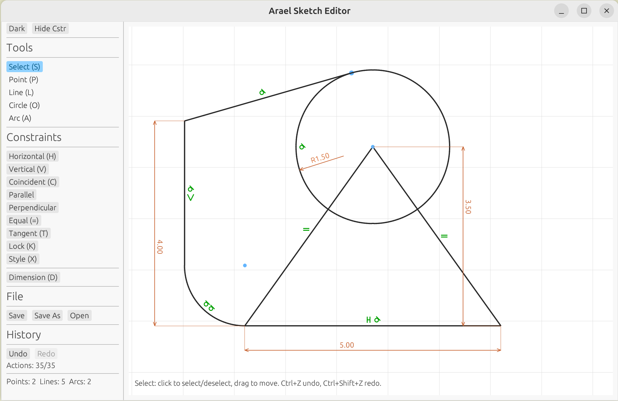
cargo expand --example slam_demo | sed -n '/fn __compute_blocks/,/^    fn /p'

§2D Sketch Editor

The arael-sketch crate provides an interactive constraint-based 2D sketch editor built on the optimization framework. It combines both differentiation modes: geometric constraints (horizontal, coincident, parallel, tangent, etc.) use compile-time differentiation, while parametric dimensions use runtime differentiation – the user types an expression like d0 * 2 + 3 and the solver constrains the geometry to satisfy it in real time, with full symbolic derivatives. Dimensions can reference each other, entity properties (L0.length, A0.radius), and arithmetic expressions, making it a fully parametric constraint solver. Runs natively and in the browser via WebAssembly.

Try it in the browser

The editor includes a command panel (/ to toggle) with 40+ scripting commands, and an embedded MCP server (--mcp) that enables AI agents like Claude Code to create and modify sketches programmatically.

Dark mode

§Example: SLAM Constraints

For multi-body optimization (SLAM, bundle adjustment), define model hierarchies with constraints. The macro handles symbolic differentiation, reference resolution, and code generation.

Hessian Sparsity

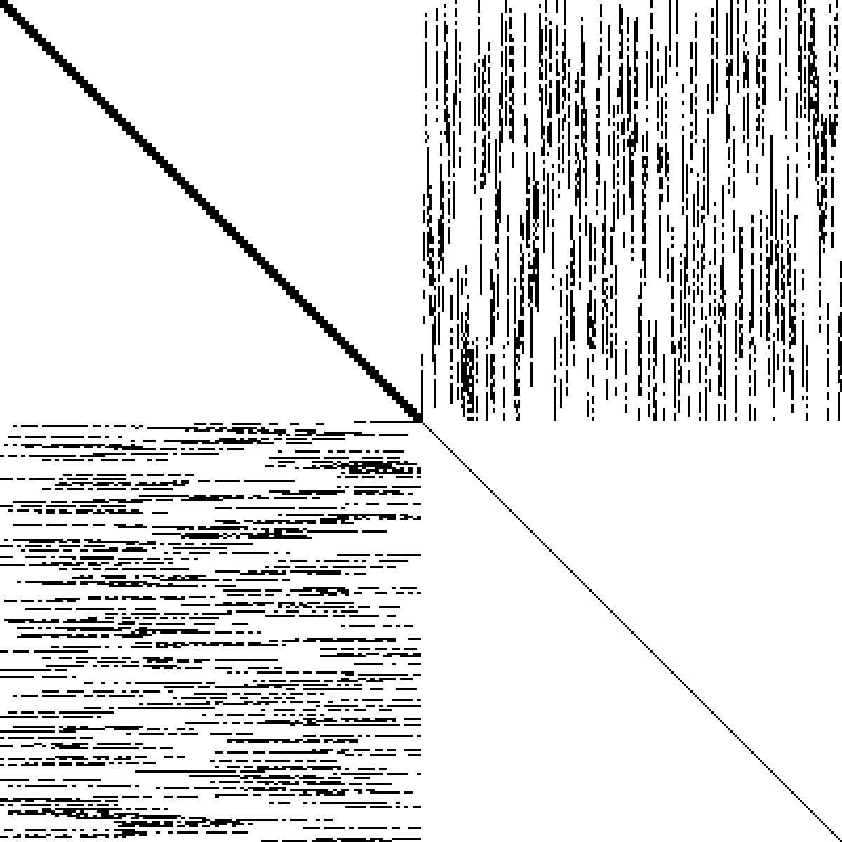
The sparsity pattern shows pose-pose blocks (upper-left), pose-landmark coupling (off-diagonal), and landmark self-blocks (lower-right). Sparse Cholesky exploits this for large speedups over dense.

#[arael::model]
#[arael(constraint(hb_pose, guard = self.info.gps.is_some(), {
    // GPS constraint (guarded -- only when data present)
    let raw = pose.pos - pose.info.gps.pos;
    let whitened = pose.info.gps.cov_r.transpose() * raw;
    [gamma * atan(whitened.x * pose.info.gps.cov_isigma.x / gamma), ...]
}))]
#[arael(constraint(hb_pose, {
    // Tilt sensor -- accelerometer constrains roll and pitch
    [(pose.ea.x - pose.info.tilt_roll) * path.tilt_isigma,
     (pose.ea.y - pose.info.tilt_pitch) * path.tilt_isigma]
}))]
struct Pose {
    pos: Param<vect3f>,
    ea: SimpleEulerAngleParam<f32>,
    info: PoseInfo,
    hb_pose: SelfBlock<Pose>,
}

// Observation linking a landmark to a pose
#[arael::model]
#[arael(constraint(hb, parent=lm, {
    let mr2w = pose.ea.rotation_matrix();
    let lm_r = mr2w.transpose() * (lm.pos - pose.pos);
    let r_f = feature.mf2r.transpose() * (lm_r - feature.camera_pos);
    [gamma * atan(atan2(r_f.y, r_f.x) * feature.isigma.x / gamma),
     gamma * atan(atan2(r_f.z, r_f.x) * feature.isigma.y / gamma)]
}))]
struct PointFrine {
    #[arael(ref = root.poses)]
    pose: Ref<Pose>,
    #[arael(ref = pose.info.features)]
    feature: Ref<PointFeature>,
    hb: CrossBlock<PointLandmark, Pose>,
}

See examples/slam_demo.rs for the full 60-pose, 240-landmark SLAM demo with GPS, odometry, tilt sensor, graduated optimization, and covariance estimation. See docs/SLAM.md for the full walkthrough.

§Starship robust error suppression

Both demos wrap every residual in $\gamma \arctan(r / \gamma)$. This is the Starship method (US Patent 12,346,118) – a way to cap how much a single outlier can move the optimum without losing smooth differentiability. This section explains what it does and why.

§Setup

Given sensor readings stacked into a vector $L$, model parameters $M$ (poses, landmarks, etc.), and a prediction $\mu(M)$ of what the sensors should report given $M$, Bayesian inference with $L \mid M \sim \mathcal{N}(\mu(M), K_L)$ – where $K_L$ is the sensor covariance matrix – leads to minimising the sum

$$ S(M) = (L - \mu(M))^T K_L^{-1} (L - \mu(M)). $$

Whitening. Diagonalising $K_L = R D R^T$ and substituting $L^D = R^T L$, $G(M) = R^T \mu(M)$ turns the quadratic form into a plain sum of squares in units of standard deviations:

$$ S(M) = \sum_i r_i^2, \qquad r_i = \frac{L_i^D - G_i(M)}{\sigma_i}. $$

The solver minimises $S(M)$ (the Gauss-Newton / LM step), and every inner term $r_i$ is dimensionless – a pure sigma count.

§The outlier problem

Each $r_i^2$ grows as the square of the measurement error. With proper covariances and no outliers a typical $|r_i|$ sits around $1$ (the whitening divides by the noise scale, so inliers cluster near unity), and $\mathbb{E}[r_i^2] = 1$ per residual. A single bad association at $10\sigma$ already contributes $100$ to the sum; at $30\sigma$ it contributes $900$. A handful of bad measurements drown out the signal from hundreds of good ones and pull the optimum off.

The usual robust-loss fixes – L1 ($|r|$) and Huber (quadratic near zero, linear past a threshold) – replace $r^2$ with something that grows slower than quadratically, which limits but does not cap each residual’s contribution; a single very bad outlier can still pull the solution. Their derivatives are also awkward: L1 has a kink at $r = 0$ (undefined derivative there), Huber has a kink at the quadratic-to-linear transition (continuous but not smooth), and Gauss-Newton wants a smooth Jacobian. We want a loss that is both fully bounded and smooth everywhere.

§The cap

We look for a function $\alpha(x)$ that behaves like $x$ in the normal range but saturates for large inputs, so that $\alpha(x)^2$ contributes a bounded amount $\Delta S_{\max}$ to the sum instead of an unbounded $x^2$.

A clean choice is

$$ \alpha(x) = \gamma \arctan\frac{x}{\gamma}, \qquad \gamma = \frac{2 \sqrt{\Delta S_{\max}}}{\pi}. $$

The $\gamma$ value follows from the saturation requirement: as $|x| \to \infty$, $\arctan(x/\gamma) \to \pm \pi/2$, so $\alpha(x)^2 \to (\gamma \pi / 2)^2$; setting that equal to $\Delta S_{\max}$ and solving gives the $\gamma$ above. Three further properties fall out:

$\alpha(x) \approx x$ for $|x| \sim 1$ – small residuals pass through unchanged.
$\alpha’(0) = 1$, so near the optimum the loss is indistinguishable from plain $r^2$.
$\alpha(x)^2 \to \Delta S_{\max}$ as $|x| \to \infty$ – no single residual can push the sum by more than $\Delta S_{\max}$.

Starship suppression function

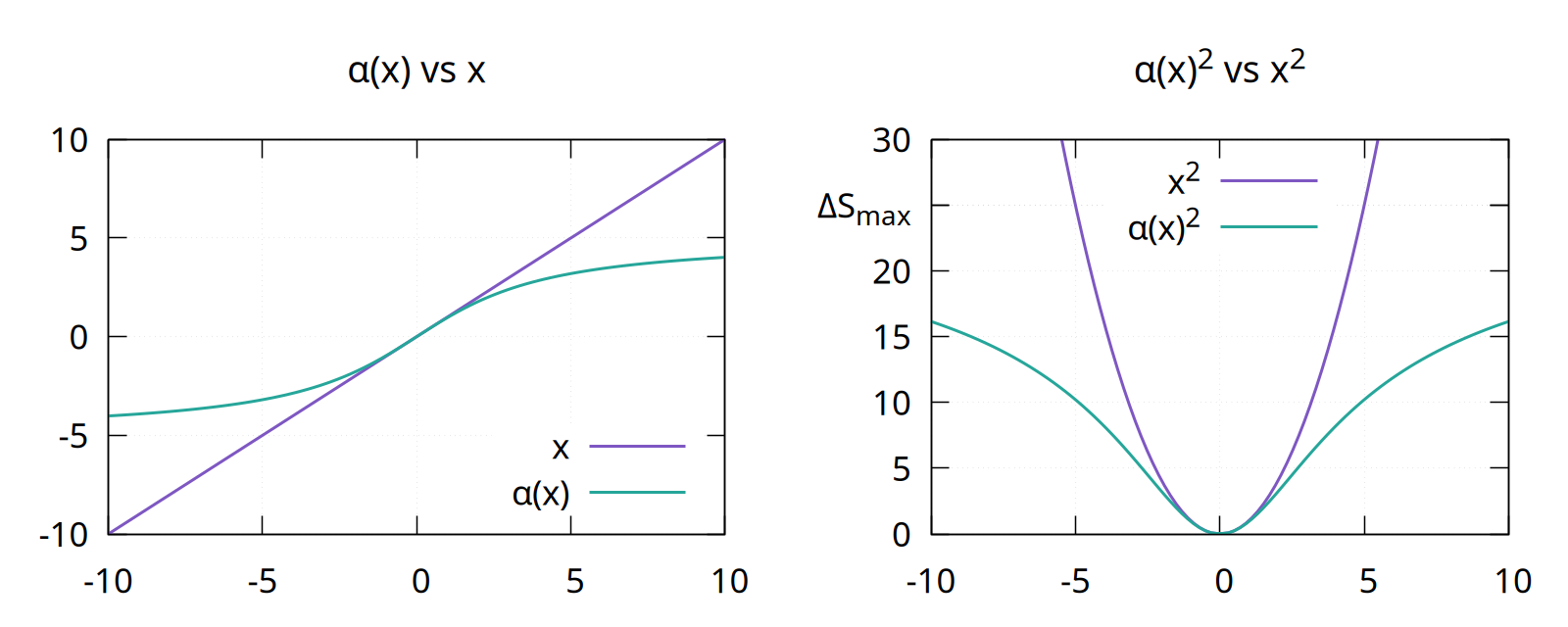
Left: $\alpha(x)$ (green) bends away from the identity $x$ (purple) once $|x|$ moves past a few sigmas. Right: the squared contribution – the unbounded $x^2$ parabola vs the saturating $\alpha(x)^2$, capped at $\Delta S_{\max}$. The cap is also smooth; Gauss-Newton still sees a well-defined Jacobian everywhere.

§Using it

Replace each $r_i$ in the sum with $\alpha(r_i)$:

$$ \hat{S}(M) = \sum_i \alpha(r_i)^2 = \sum_i \left[ \gamma \arctan\frac{L_i^D - G_i(M)}{\gamma \sigma_i} \right]^2. $$

In practice $\Delta S_{\max}$ in the range $[10, 25]$ (so $\gamma$ between roughly $2$ and $3$) suppresses genuine outliers hard without biasing inlier-dominated regions. Since residuals are already sigma-scaled, this corresponds roughly to saying “residuals past $3$ to $5\sigma$ stop mattering”.

In arael this is exactly what you see in the demo constraint bodies:

let plain_r = (a * e.x + b - e.y) / sigma;
gamma * atan(plain_r / gamma)

The symbolic-differentiation pipeline handles atan’s derivative automatically; from the macro’s point of view the residual is just another expression. No special-case code, no outlier bookkeeping.

§Initialisation matters

Gauss-Newton (and Levenberg-Marquardt) is a local method: each step linearises the cost around the current $M$ and moves in the direction that linearisation suggests. For any loss, you need a starting $M_0$ close enough to the optimum that the linearisation is informative.

Starship makes this requirement stricter. The gradient falls off as $\alpha’(r) = 1 / (1 + \pi^2 r^2 / (4 \Delta S_{\max}))$, so at the recommended $\Delta S_{\max} = 25$ a residual at $5\sigma$ still carries about 29% of its least-squares pull and a $10\sigma$ residual about 9% – still usable. Once you get out to $20\sigma$ and beyond it drops under 3% and those residuals are effectively frozen. If $M_0$ puts many residuals that far out, the solver has nothing to work with and stalls. The usual remedy is graduated optimisation: start with a large $\Delta S_{\max}$ (loose cap, everything in the informative regime), solve, then shrink it across passes down to the target value. The SLAM demo does this via a frine_isigma_scale field stepped per pass.

§Example: Localization

Same model as SLAM but landmarks are fixed (known map). With only pose parameters the hessian is block-tridiagonal, so the band solver gives O(n) scaling – 9.4x faster than dense at 500 poses. See examples/loc_demo.rs.

§Examples

The examples/ directory is the primary place to see the API in use. Each file is a runnable cargo run --release --example <name>.

bench_band – benchmarks the band Cholesky backend against dense on the localisation model at increasing pose counts. Prints timing + speedup.
bench_investigate – deeper comparison of sparse backends (faer, schur) on the SLAM model, with assembly vs solve breakdown and numeric cross-check of the solutions.
bench_sparse – sparse Cholesky backends (faer / schur) vs dense on SLAM.
calc_demo – bc-style REPL calculator built on arael-sym. Shows parse_with_functions + FunctionBag for user-defined functions, persistent history via rustyline.
jacobian_demo – #[arael(root, jacobian)], #[arael(constraint_index)], and calc_jacobian / calc_cost_table walk-through. End-to-end reference for the instrumentation features referenced from “My solve doesn’t converge”.
linear_demo – robust linear regression on noisy 2D data. Residual wrapped in gamma * atan(r / gamma) – the Starship method (US12346118), same robustifier used by the feature constraints in loc/SLAM. Minimal single-struct model + LM fit, compared against plain closed-form least squares.
loc_demo – localisation with fixed known landmarks (no gauge freedom). Block-tridiagonal Hessian + band solver. Graduated-isigma optimisation via a root frine_isigma_scale field.
loc_global_demo – how to put Param fields on the root struct and have constraints consume them. Uses a system-global rigid transform (translation + 3-axis rotation applied to every pose) as the running example; every residual that reads the robot’s world pose composes the globals before evaluating. Shows the two wiring shapes for pose<->root cross-Hessian pairs (CrossBlock<Pose, Path> on the constraint struct, and a root-owned TripletBlock named via the root.<field> block spec) and a Path::optimise_center pass that freezes pose params and optimises only the globals before the main sweep.
model_demo – minimal #[arael::model] walk-through showing how Param, SimpleEulerAngleParam, and the update cycle fit together.
refs_demo – Ref<T>, refs::Vec, refs::Deque, and refs::Arena behaviour: insertion, iteration, stable handles.
runtime_fit_demo – curve fitting where the residual equation is a string parsed at runtime. Demonstrates ExtendedModel + robust loss on top of the symbolic front end.
single_root_demo – single-struct model-and-root + a direct-composed sub-model, each carrying its own SelfBlock<Self>. The smallest example that exercises the “root has its own params” path.
slam_demo – synthetic visual-inertial SLAM: S-curve trajectory, 20 poses, 40 landmarks, odometry + tilt + GPS + feature observations. Full verbose-LM trace across graduated isigma passes – the reference for what a healthy solver run looks like.
sym_demo – symbolic-math tour: expression building, automatic differentiation, CSE, pretty printing, parsing. No solver involvement; pure arael-sym.
user_function_demo – #[arael::function] for user-defined operators in constraint bodies. Form A purely symbolic sigmoid(x) = 1 / (1 + exp(-x)) and Form B opaque numerical my_safe_asin with a closed-form symbolic derivative, both used in a single two-residual LM fit.

§Crate structure

arael-sym – symbolic math engine (expression trees, differentiation, CSE)
arael-macros – proc macros (#[arael::model], #[derive(Model)])
arael (this crate) – runtime: model traits, solvers, geometry, vectors

Re-exports§

pub use model::Jacobian;
pub use model::JacobianRow;
pub use model::jacobian_entries;
pub use arael_sym as sym;

Modules§

geometry: Camera model and geometric utilities. Geometric primitives for camera models and projections.
matrix: 3x3 and 2x2 matrix types with rotation and linear algebra. 2x2 and 3x3 matrix types with rotation, transpose, and linear algebra operations.
model: Model trait, parameter types, and Hessian blocks.
quatern: Quaternion type for 3D rotations. Quaternion type for 3D rotations.
refs: Type-safe indexed collections: Ref, Vec, Deque, Arena. Type-safe indexed collections with stable Ref-based access.
simple_lm: Levenberg-Marquardt solver with dense, band, and sparse backends. Levenberg-Marquardt solver with dense, band, and sparse backends.
user_fn: Runtime registry for user-defined functions declared via #[arael::function]. Built from inventory submissions; see user_fn::registry_bag. Runtime registry for user-defined functions declared via #[arael::function]. Populated at program start via inventory, consulted by the emitted sibling fns so calls like sigmoid(x) or my_safe_asin(x) from ordinary Rust can resolve every other registered user function (including forward references and mutual recursion).
utils: Numeric traits (Float). Numeric traits and angle utilities.
vect: 2D and 3D vector types. 2D and 3D vector types with standard math operations.

Macros§

error: Log an error message to stderr.
info: Log an informational message to stderr.
sym: The sym! auto-clone macro for symbolic expressions (from arael-sym). Auto-clone macro for symbolic math expressions.
warn: Log a warning message to stderr.

Attribute Macros§

function: Attribute macro: #[arael::function]. Register a user-defined function for use in #[arael::model] constraint bodies. Two forms:
model: Attribute macro: #[arael::model]. Attribute macro for arael model structs.

Derive Macros§

Model: Derive macro for the Model trait.

Crate arael

Crate arael Copy item path

§Contents

§Features

§Scope

§Example: Symbolic Math

§Example: Robust Linear Regression

§Runtime Differentiation

§Model Structure

§Parameter types

§Initial values via the _value suffix

§Parameter control

§Hessian block types

§Multi-CrossBlock vs TripletBlock

§Collection types

§Struct-level macro attributes

§Constraint attributes

§Field-level macro attributes

§User-defined functions (#[arael::function])

§Form A: purely symbolic

§Form B: opaque numerical eval + symbolic derivatives

§Ergonomics

§Runtime differentiation (ExtendedModel)

§Solvers

§Which backend?

§Basic usage

§LmConfig – every field, with defaults

§Tuning for performance vs quality

§At the very top end

§LM in five bullets

§Verbose trace format

§Graduated optimisation

§Instrumentation & Debugging

§My solve doesn’t converge. What do I check?

§How do I know my new constraint is actually doing anything?

§Looking under the hood with cargo expand

§Example: a one-line fix constraint

§Example: shared subexpressions

§What to look for

§2D Sketch Editor

§Example: SLAM Constraints

§Starship robust error suppression

§Setup

§The outlier problem

§The cap

§Using it

§Initialisation matters

§Example: Localization

§Examples

§Crate structure

Re-exports§

Modules§

Macros§

Attribute Macros§

Derive Macros§

Crate arael

§Initial values via the `_value` suffix

§User-defined functions (`#[arael::function]`)

§Runtime differentiation (`ExtendedModel`)

§`LmConfig` – every field, with defaults

§Looking under the hood with `cargo expand`